1. Cluster/Group Analysis
Cluster Analysis allows data to be grouped using two types of methods: Hierarchical or K-means.
For the hierarchical method, you can choose the distance parameters (Euclidean, Manhattan or Gower) and the method (ward, single, complete, average, median or centroid). There are options to standardize the data, display the data in a dendrogram and display groups.
For the K-means method there is only the possibility of defining the number of groups and standardizing the data.
Example 1:
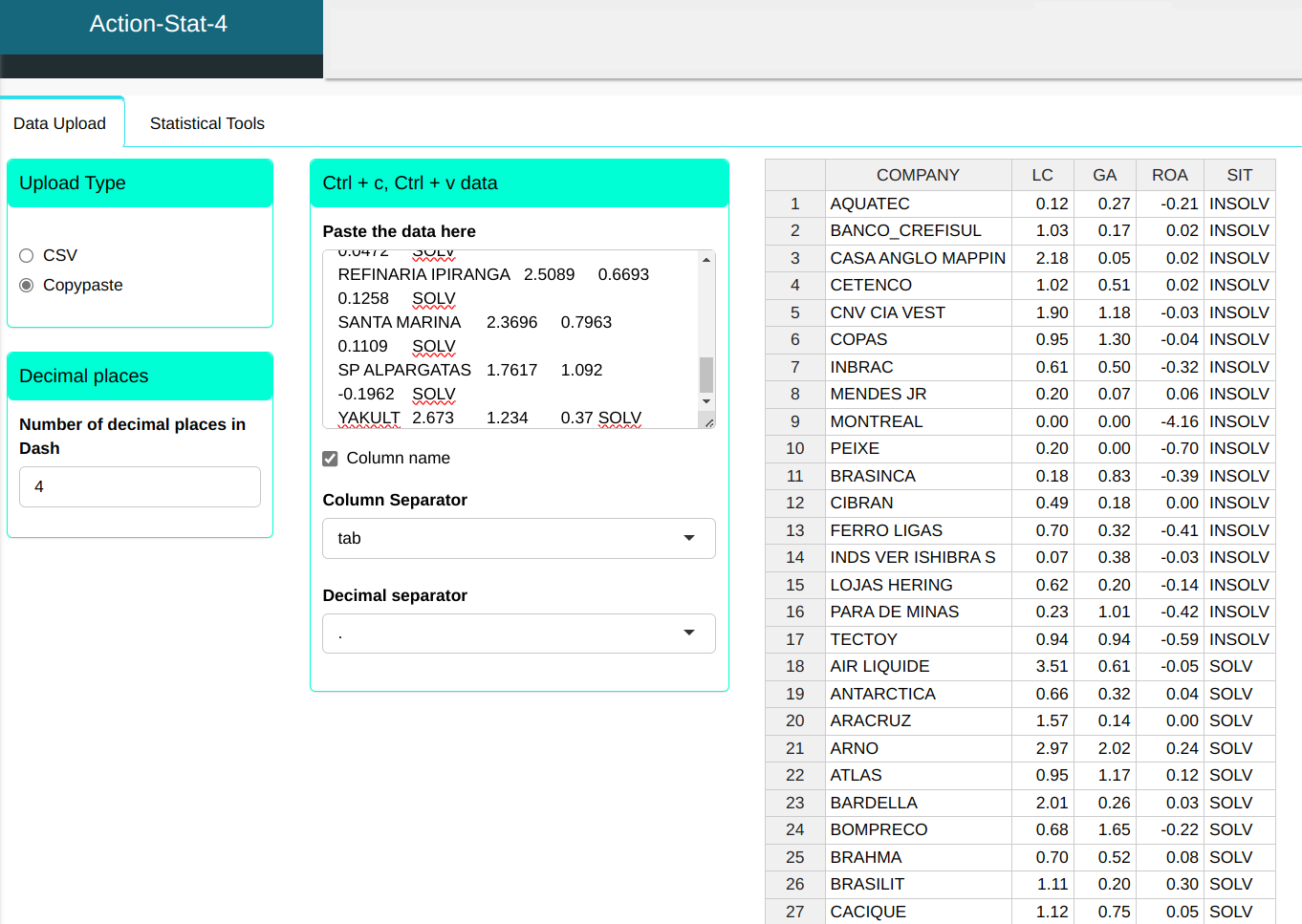
A financial analyst would like to segment the companies analyzed according to the factors that impact their financial health. The consumer goods manufacturer, after mapping the market structure and determining the factors that differentiate the products, would like to segment them. We will apply Cluster Analysis using the hierarchical complete linkage method using Euclidean distance to compare groups.
The mapped factors are shown in the table below.
| COMPANY | LC | GA | ROA | SIT |
|---|---|---|---|---|
| AQUATEC | 0.1159 | 0.2673 | -0.2101 | INSOLV |
| BANCO_CREFISUL | 1.0317 | 0.1721 | 0.0196 | INSOLV |
| CASA ANGLO MAPPIN | 2.1758 | 0.0456 | 0.0179 | INSOLV |
| CETENCO | 1.0213 | 0.5076 | 0.0178 | INSOLV |
| CNV CIA VEST | 1.9036 | 1.1809 | -0.0283 | INSOLV |
| COPAS | 0.9484 | 1.3017 | -0.0434 | INSOLV |
| INBRAC | 0.6121 | 0.4972 | -0.3229 | INSOLV |
| MENDES JR | 204 | 0.0667 | 0.0561 | INSOLV |
| MONTREAL | 0.0045 | 0 | -4.1594 | INSOLV |
| PEIXE | 0.2049 | 0 | -0.7039 | INSOLV |
| BRASINCA | 0.1775 | 0.8322 | -0.3944 | INSOLV |
| CIBRAN | 0.4855 | 0.1843 | -0.0048 | INSOLV |
| FERRO LIGAS | 0.6955 | 0.3195 | -0.4052 | INSOLV |
| INDS VER ISHIBRA S | 0.0683 | 0.3828 | -0.0293 | INSOLV |
| LOJAS HERING | 0.6238 | 0.1983 | -0.1372 | INSOLV |
| PARA DE MINAS | 0.2326 | 1014 | -0.4158 | INSOLV |
| TECTOY | 0.9442 | 0.9431 | -0.5884 | INSOLV |
| AIR LIQUIDE | 3.5053 | 0.6109 | -0.0464 | SOLV |
| ANTARCTICA | 0.6613 | 0.3192 | 0.0379 | SOLV |
| ARACRUZ | 1.5707 | 0.1427 | 1 | SOLV |
| ARNO | 2.9656 | 2.0212 | 0.2423 | SOLV |
| ATLAS | 0.9515 | 1.1676 | 0.1214 | SOLV |
| BARDELLA | 2.0071 | 0.2559 | 0.0276 | SOLV |
| BOMPRECO | 0.6804 | 1.6503 | -0.2219 | SOLV |
| BRAHMA | 0.7031 | 0.5195 | 0.0797 | SOLV |
| BRASILIT | 1105 | 0.1958 | 0.2984 | SOLV |
| CACIQUE | 1.1209 | 748 | 0.0464 | SOLV |
| CONFAB TUBOS | 2266 | 0.3392 | 98 | SOLV |
| DURATEX | 2.4744 | 0.4178 | 0.0647 | SOLV |
| EBERLE | 0.4188 | 1.1136 | -0.1495 | SOLV |
| EMBRACO | 1.7798 | 0.7221 | 0.0558 | SOLV |
| ENGEMIX | 1.2954 | 1.2006 | 0.0345 | SOLV |
| ERICSSON | 1.6473 | 629 | 0.1568 | SOLV |
| FICAP | 2.3485 | 1.4813 | 0.1218 | SOLV |
| GERDAU | 1.2619 | 0.3317 | 0.0381 | SOLV |
| LPC DANONE | 1.4377 | 2.3197 | 0.1207 | SOLV |
| MAGNESITA | 1.7495 | 0.7416 | 0.0576 | SOLV |
| MILLENNIUM | 0.9254 | 0.4134 | -0.0289 | SOLV |
| MONARK | 1.9217 | 0.8222 | 0.1926 | SOLV |
| MULTIBRA S | 1.7066 | 1.2666 | 0.2244 | SOLV |
| NADIR FIGUEIREDO | 1.5415 | 826 | 0.0058 | SOLV |
| NITROCARBONO | 0.7424 | 0.9485 | 0.0401 | SOLV |
| PETTENATI | 1.4648 | 0.6864 | 0.2433 | SOLV |
| PIRELLI PNEUS | 1.3069 | 1452 | 0.1059 | SOLV |
| PRONOR PETROQ | 758 | 499 | 0.0472 | SOLV |
| REFINARIA IPIRANGA | 2.5089 | 0.6693 | 0.1258 | SOLV |
| SANTA MARINA | 2.3696 | 0.7963 | 0.1109 | SOLV |
| SP ALPARGATAS | 1.7617 | 1092 | -0.1962 | SOLV |
| YAKULT | 2673 | 1234 | 0.37 | SOLV |
We will upload the data to the system.
Configuring as shown in the figure below to perform the analysis of clustering.
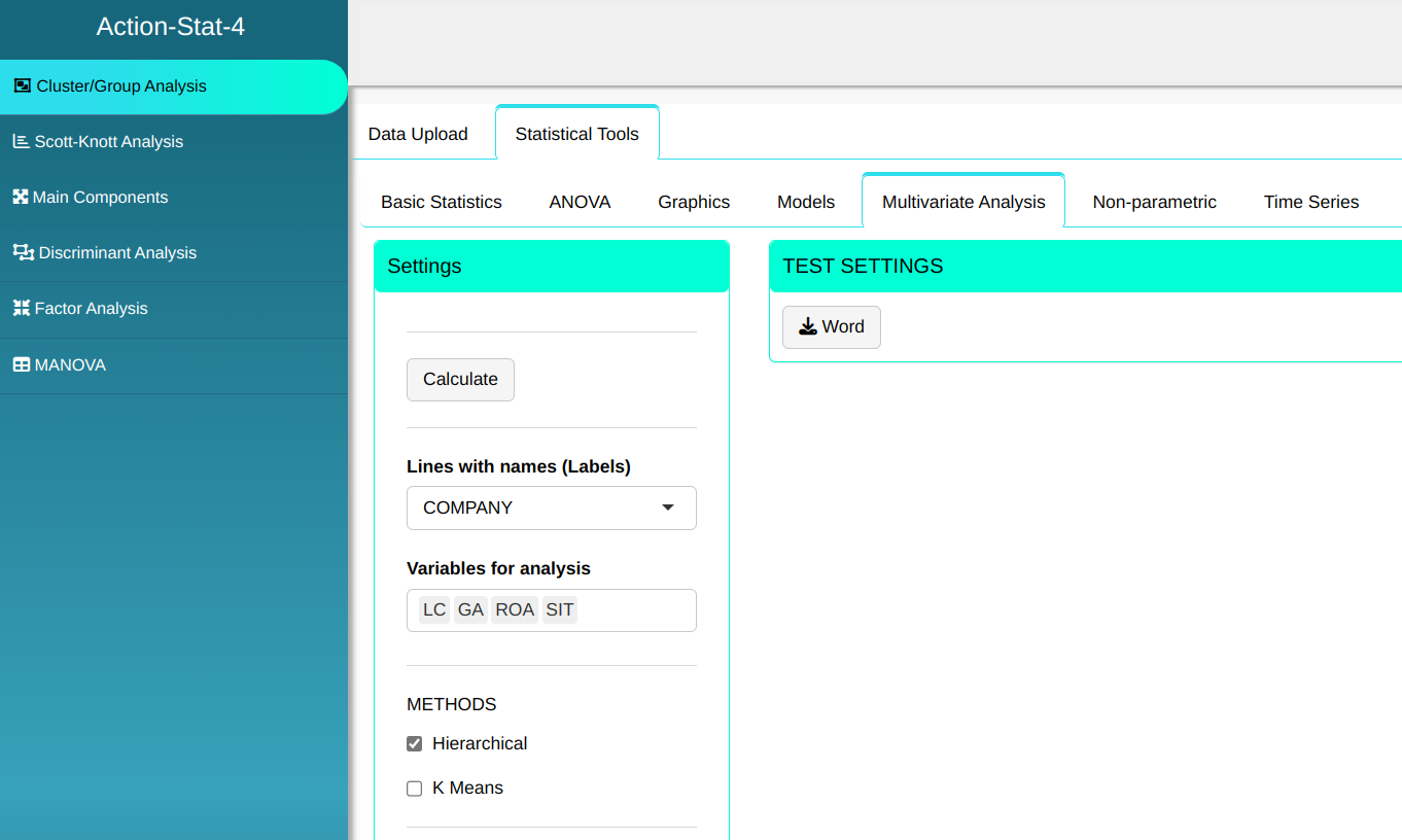
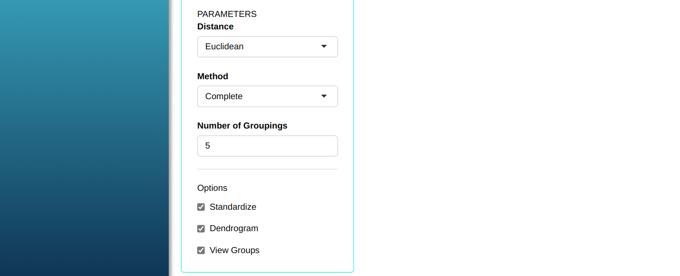
Then click Calculate to get the results. You can also generate the analyses and download them in Word format.

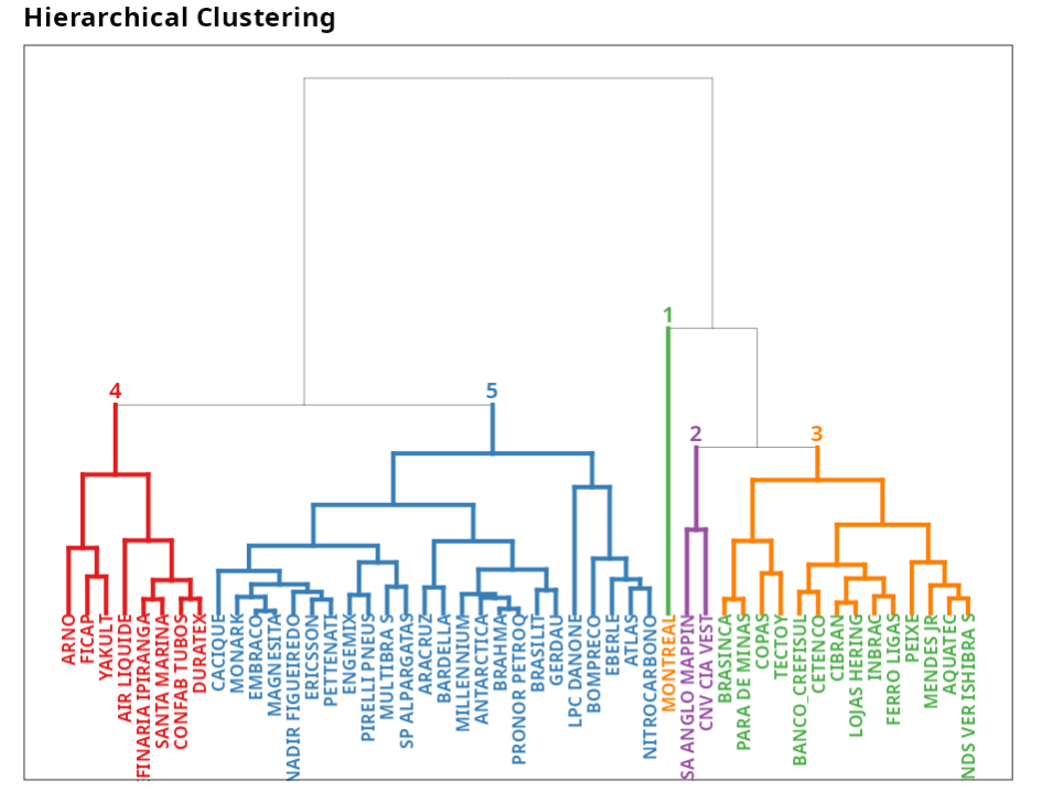
The results are:
hierarchical Clustering
| Group 1 | Group 2 | Group 3 | Group 4 | Group 5 |
|---|---|---|---|---|
| AQUATEC | CASA ANGLO (MAPPIN) | MONTREAL | AIR LIQUIDE | ANTARCTICA |
| BANCO_CREFISUL | CNV CIA VEST | ARNO | ARACRUZ | |
| CETENCO | CONFAB TUBOS | ATLAS | ||
| COPAS | DURATEX | BARDELLA | ||
| INBRAC | FICAP | BOMPREÇO | ||
| MENDES JR. | REFINARIA IPIRANGA | BRAHMA | ||
| PEIXE | SANTA MARINA | BRASILIT | ||
| BRASINCA | YAKULT | CACIQUE | ||
| CIBRAN | EBERLE | |||
| FERRO LIGAS | EMBRACO | |||
| INDS.VER.ISHIBRA´S | ENGEMIX | |||
| LOJAS HERING | ERICSSON | |||
| PARA DEMINAS | GERDAU | |||
| TECTOY | LPC(DANONE) | |||
| MAGNESITA | ||||
| MILLENNIUM | ||||
| MONARK | ||||
| MULTIBRA´S | ||||
| NADIR | ||||
| FIGUEIREDO | ||||
| NITROCARBONO | ||||
| PETTENATI | ||||
| PIRELLI PNEUS | ||||
| PRONOR PETROQ. | ||||
| SP ALPARGATAS |
Group
| Labels | Residual Order | Groups |
|---|---|---|
| AQUATEC | 1 | 1 |
| BANCO_CREFISUL | 2 | 1 |
| CASA ANGLO (MAPPIN) | 3 | 2 |
| CETENCO | 4 | 1 |
| CNV CIA VEST | 5 | 2 |
| COPAS | 6 | 1 |
| INBRAC | 7 | 1 |
| MENDES JR. | 8 | 1 |
| MONTREAL | 9 | 3 |
| PEIXE | 10 | 1 |
| BRASINCA | 11 | 1 |
| CIBRAN | 12 | 1 |
| FERRO LIGAS | 13 | 1 |
| INDS.VER.ISHIBRA´S | 14 | 1 |
| LOJAS HERING | 15 | 1 |
| PARA DEMINAS | 16 | 1 |
| TECTOY | 17 | 1 |
| AIR LIQUIDE | 18 | 4 |
| ANTARCTICA | 19 | 5 |
| ARACRUZ | 20 | 5 |
| ARNO | 21 | 4 |
| ATLAS | 22 | 5 |
| BARDELLA | 23 | 5 |
| BOMPREÇO | 24 | 5 |
| BRAHMA | 25 | 5 |
| BRASILIT | 26 | 5 |
| CACIQUE | 27 | 5 |
| CONFAB TUBOS | 28 | 4 |
| DURATEX | 29 | 4 |
| EBERLE | 30 | 5 |
| EMBRACO | 31 | 5 |
| ENGEMIX | 32 | 5 |
| ERICSSON | 33 | 5 |
| FICAP | 34 | 4 |
| GERDAU | 35 | 5 |
| LPC(DANONE) | 36 | 5 |
| MAGNESITA | 37 | 5 |
| MILLENNIUM | 38 | 5 |
| MONARK | 39 | 5 |
| MULTIBRA´S | 40 | 5 |
| NADIR FIGUEIREDO | 41 | 5 |
| NITROCARBONO | 42 | 5 |
| PETTENATI | 43 | 5 |
| PIRELLI PNEUS | 44 | 5 |
| PRONOR PETROQ. | 45 | 5 |
| REFINARIA IPIRANGA | 46 | 4 |
| SANTA MARINA | 47 | 4 |
| SP ALPARGATAS | 48 | 5 |
| YAKULT | 49 | 4 |
Example 2:
Consider the monthly income (in minimum wages) and age of six individuals in a given location. We will apply Cluster Analysis using the hierarchical method of linking means using Euclidean distance to compare the groups.
| Individual | Rent | Age |
|---|---|---|
| A | 9.6 | 28 |
| B | 8.4 | 31 |
| C | 2.4 | 42 |
| D | 18.2 | 38 |
| E | 3.9 | 25 |
| F | 6.4 | 41 |
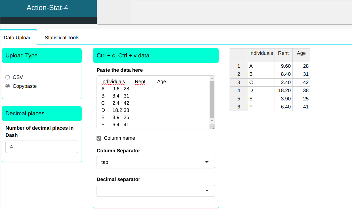
Configuring as shown in the figure below to perform the analysis of clustering.
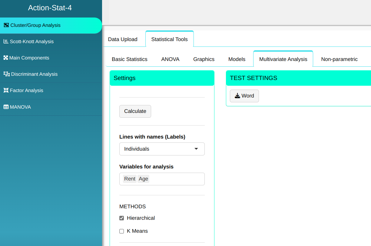
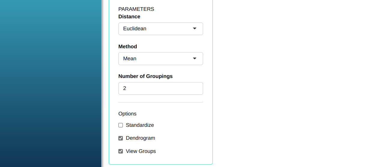
Then click Calculate to get the results. You can also generate the analyses and download them in Word format.
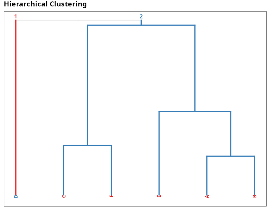
The results are:
Hierarchical Clustering
| Group 1 | Group 2 |
|---|---|
| A | D |
| B | |
| C | |
| E | |
| F |
Group
| Labels | Residual Order | Group |
|---|---|---|
| A | 1 | 1 |
| B | 2 | 1 |
| C | 3 | 1 |
| D | 4 | 2 |
| E | 5 | 1 |
| F | 6 | 1 |
Example 3:
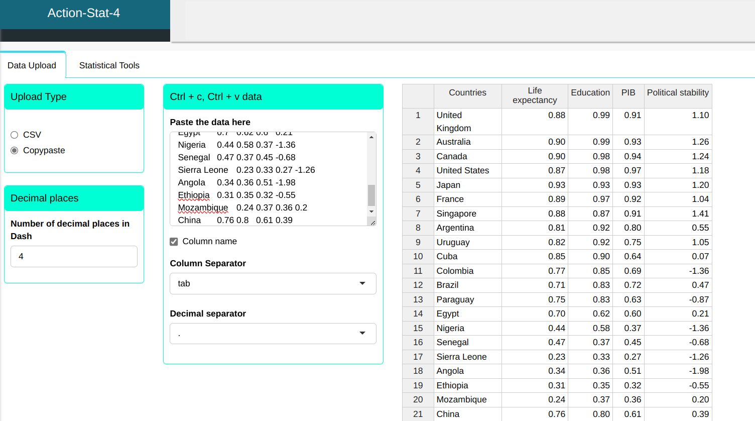
The data represents, according to the UN database (2002), the life expectancy, education, income (GDP) and political stability and security indices of 21 countries. The higher the index value, the better the quality of the country. We will apply Cluster Analysis using the hierarchical method using Euclidean distance with Ward’s method to compare the groups.
Let us upload the data into the system.
| Countries | Life expectancy | Education | PIB | Political stability |
|---|---|---|---|---|
| United Kingdom | 0.88 | 0.99 | 0.91 | 1.1 |
| Australia | 0.9 | 0.99 | 0.93 | 1.26 |
| Canada | 0.9 | 0.98 | 0.94 | 1.24 |
| United States | 0.87 | 0.98 | 0.97 | 1.18 |
| Japan | 0.93 | 0.93 | 0.93 | 1.2 |
| France | 0.89 | 0.97 | 0.92 | 1.04 |
| Singapore | 0.88 | 0.87 | 0.91 | 1.41 |
| Argentina | 0.81 | 0.92 | 0.8 | 0.55 |
| Uruguay | 0.82 | 0.92 | 0.75 | 1.05 |
| Cuba | 0.85 | 0.9 | 0.64 | 0.07 |
| Colombia | 0.77 | 0.85 | 0.69 | -1.36 |
| Brazil | 0.71 | 0.83 | 0.72 | 0.47 |
| Paraguay | 0.75 | 0.83 | 0.63 | -0.87 |
| Egypt | 0.7 | 0.62 | 0.6 | 0.21 |
| Nigeria | 0.44 | 0.58 | 0.37 | -1.36 |
| Senegal | 0.47 | 0.37 | 0.45 | -0.68 |
| Sierra Leone | 0.23 | 0.33 | 0.27 | -1.26 |
| Angola | 0.34 | 0.36 | 0.51 | -1.98 |
| Ethiopia | 0.31 | 0.35 | 0.32 | -0.55 |
| Mozambique | 0.24 | 0.37 | 0.36 | 0.2 |
| China | 0.76 | 0.8 | 0.61 | 0.39 |
Configuring as shown in the figure below to perform the analysis of clustering.
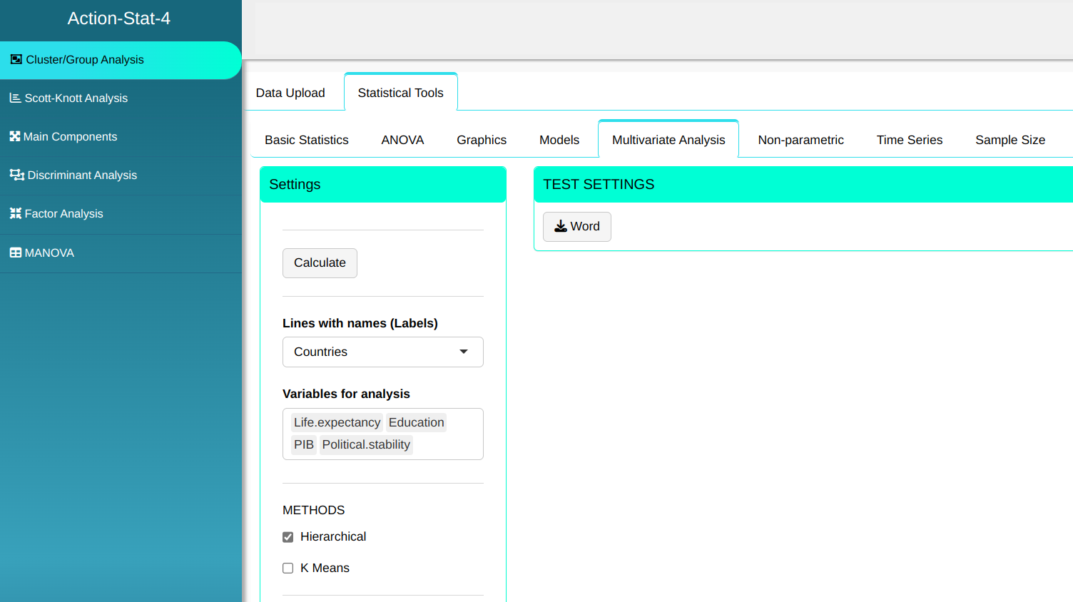
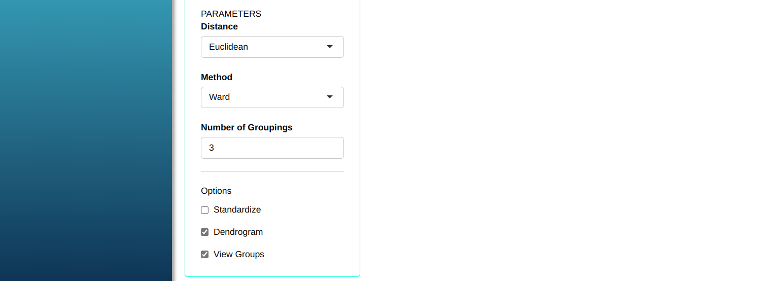
Then click Calculate to get the results. You can also generate the analyses and download them in Word format.
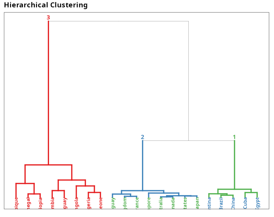
The results are:são:
Hierarchical Clustering
| Group 1 | Group 2 | Group 3 |
|---|---|---|
| United Kingdom | Argentina | Colombia |
| Australia | Cuba | Paraguay |
| Canada | Brazil | Nigeria |
| United States | Egypt | Senegal |
| Japan | China | Sierra Leone |
| France | Angola | |
| Singapore | Ethiopia | |
| Uruguay | Mozambique |
Group
| Labels | Residual Order | Groups | |
|---|---|---|---|
| 1 | United Kingdom | 1 | 1 |
| 2 | Australia | 2 | 1 |
| 3 | Canada | 3 | 1 |
| 4 | United States | 4 | 1 |
| 5 | Japan | 5 | 1 |
| 6 | France | 6 | 1 |
| 7 | Singapore | 7 | 1 |
| 8 | Argentina | 8 | 2 |
| 9 | Uruguay | 9 | 1 |
| 10 | Cuba | 10 | 2 |
| 11 | Colombia | 11 | 3 |
| 12 | Brazil | 12 | 2 |
| 13 | Paraguay | 13 | 3 |
| 14 | Egypt | 14 | 2 |
| 15 | Nigeria | 15 | 3 |
| 16 | Senegal | 16 | 3 |
| 17 | Sierra Leone | 17 | 3 |
| 18 | Angola | 18 | 3 |
| 19 | Ethiopia | 19 | 3 |
| 20 | Mozambique | 20 | 3 |
| 21 | China | 21 | 2 |
Example 4:
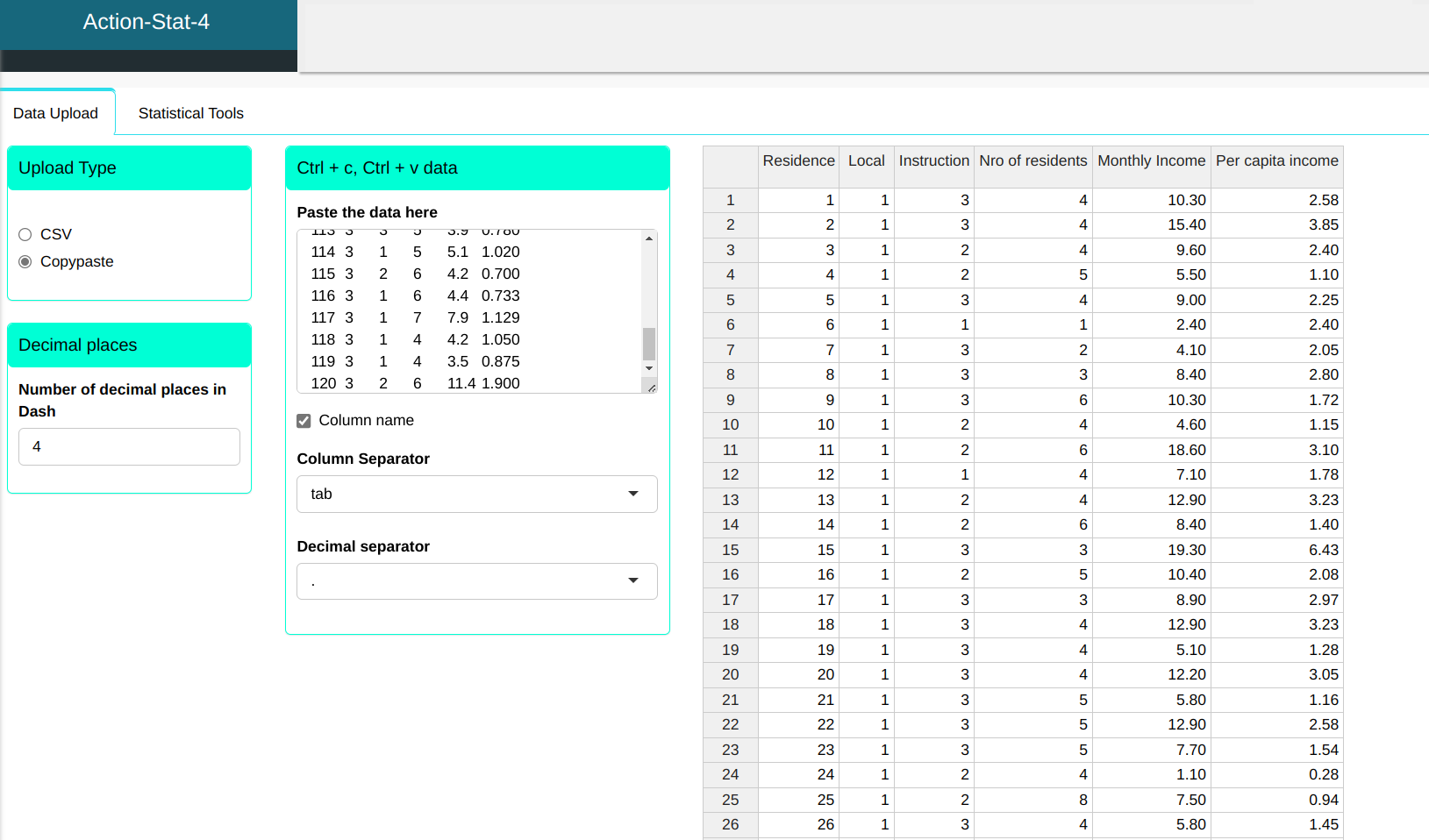
It is common to use stratified random sampling when collecting survey data. The table below shows data from a survey of 120 households in a given region, measuring five variables: the location of the household, the level of education of the head of the household, the number of people living in the household, the monthly household income in minimum wages and the monthly household income per capita. We will use cluster analysis to help define these strata, employing the hierarchical method using the Manhattan distance with Ward’s method for group comparison.
| Residence | Local | Instruction | Nro of Residents | Monthly Income | Per capita income |
|---|---|---|---|---|---|
| 1 | 1 | 3 | 4 | 10.3 | 2.575 |
| 2 | 1 | 3 | 4 | 15.4 | 3.850 |
| 3 | 1 | 2 | 4 | 9.6 | 2.400 |
| 4 | 1 | 2 | 5 | 5.5 | 1.100 |
| 5 | 1 | 3 | 4 | 9 | 2.250 |
| 6 | 1 | 1 | 1 | 2.4 | 2.400 |
| 7 | 1 | 3 | 2 | 4.1 | 2.050 |
| 8 | 1 | 3 | 3 | 8.4 | 2.800 |
| 9 | 1 | 3 | 6 | 10.3 | 1.717 |
| 10 | 1 | 2 | 4 | 4.6 | 1.150 |
| 11 | 1 | 2 | 6 | 18.6 | 3.100 |
| 12 | 1 | 1 | 4 | 7.1 | 1.775 |
| 13 | 1 | 2 | 4 | 12.9 | 3.225 |
| 14 | 1 | 2 | 6 | 8.4 | 1.400 |
| 15 | 1 | 3 | 3 | 19.3 | 6.433 |
| 16 | 1 | 2 | 5 | 10.4 | 2.080 |
| 17 | 1 | 3 | 3 | 8.9 | 2.967 |
| 18 | 1 | 3 | 4 | 12.9 | 3.225 |
| 19 | 1 | 3 | 4 | 5.1 | 1.275 |
| 20 | 1 | 3 | 4 | 12.2 | 3.050 |
| 21 | 1 | 3 | 5 | 5.8 | 1.160 |
| 22 | 1 | 3 | 5 | 12.9 | 2.580 |
| 23 | 1 | 3 | 5 | 7.7 | 1.540 |
| 24 | 1 | 2 | 4 | 1.1 | 0.275 |
| 25 | 1 | 2 | 8 | 7.5 | 0.938 |
| 26 | 1 | 3 | 4 | 5.8 | 1.450 |
| 27 | 1 | 1 | 5 | 7.2 | 1.440 |
| 28 | 1 | 3 | 3 | 8.6 | 2.867 |
| 29 | 1 | 2 | 4 | 5.1 | 1.275 |
| 30 | 1 | 3 | 5 | 2.6 | 0.520 |
| 31 | 1 | 3 | 5 | 7.7 | 1.540 |
| 32 | 1 | 2 | 2 | 2.4 | 1.200 |
| 33 | 1 | 3 | 5 | 4.8 | 0.960 |
| 34 | 1 | 1 | 2 | 2.1 | 1.050 |
| 35 | 1 | 1 | 6 | 4 | 0.667 |
| 36 | 1 | 1 | 8 | 12.5 | 1.563 |
| 37 | 1 | 3 | 3 | 6.8 | 2.267 |
| 38 | 1 | 3 | 5 | 3.9 | 0.780 |
| 39 | 1 | 3 | 5 | 9 | 1.800 |
| 40 | 1 | 3 | 3 | 10.9 | 3.633 |
| 41 | 2 | 2 | 5 | 5.4 | 1.080 |
| 42 | 2 | 1 | 3 | 6.4 | 2.133 |
| 43 | 2 | 1 | 6 | 4.4 | 0.733 |
| 44 | 2 | 1 | 5 | 2.5 | 0.500 |
| 45 | 2 | 1 | 6 | 5.5 | 0.917 |
| 46 | 2 | 1 | 8 | 4.8 | 0.600 |
| 47 | 2 | 3 | 4 | 14 | 3.500 |
| 48 | 2 | 2 | 4 | 8.5 | 2.125 |
| 49 | 2 | 1 | 5 | 7.7 | 1.540 |
| 50 | 2 | 2 | 3 | 5.8 | 1.933 |
| 51 | 2 | 3 | 5 | 5 | 1.000 |
| 52 | 2 | 1 | 3 | 4.8 | 1.600 |
| 53 | 2 | 2 | 2 | 2.8 | 1.400 |
| 54 | 2 | 2 | 4 | 4.2 | 1.050 |
| 55 | 2 | 3 | 3 | 10.2 | 3.400 |
| 56 | 2 | 2 | 4 | 7.4 | 1.850 |
| 57 | 2 | 2 | 5 | 5 | 1.000 |
| 58 | 2 | 3 | 2 | 6.4 | 3.200 |
| 59 | 2 | 3 | 4 | 5.7 | 1.425 |
| 60 | 2 | 2 | 4 | 10.8 | 2.700 |
| 61 | 2 | 3 | 1 | 2.3 | 2.300 |
| 62 | 2 | 1 | 7 | 6.1 | 0.871 |
| 63 | 2 | 1 | 3 | 5.5 | 1.833 |
| 64 | 2 | 1 | 7 | 3.5 | 0.500 |
| 65 | 2 | 3 | 3 | 9 | 3.000 |
| 66 | 2 | 3 | 6 | 5.8 | 0.967 |
| 67 | 2 | 1 | 6 | 4.2 | 0.700 |
| 68 | 2 | 3 | 3 | 6.8 | 2.267 |
| 69 | 2 | 2 | 5 | 4.8 | 0.960 |
| 70 | 2 | 3 | 5 | 6 | 1.200 |
| 71 | 2 | 2 | 7 | 9 | 1.286 |
| 72 | 2 | 1 | 4 | 5.3 | 1.325 |
| 73 | 2 | 3 | 4 | 3.1 | 0.775 |
| 74 | 2 | 3 | 1 | 6.4 | 6.400 |
| 75 | 2 | 1 | 3 | 3.9 | 1.300 |
| 76 | 2 | 2 | 3 | 6.4 | 2.133 |
| 77 | 2 | 3 | 4 | 2.7 | 0.675 |
| 78 | 2 | 2 | 4 | 2.4 | 0.600 |
| 79 | 2 | 2 | 4 | 3.6 | 0.900 |
| 80 | 2 | 3 | 5 | 6.4 | 1.280 |
| 81 | 2 | 3 | 2 | 11.3 | 5.650 |
| 82 | 2 | 1 | 5 | 3.8 | 0.760 |
| 83 | 2 | 2 | 3 | 4.1 | 1.367 |
| 84 | 3 | 1 | 5 | 1.8 | 0.360 |
| 85 | 3 | 3 | 5 | 7.1 | 1.420 |
| 86 | 3 | 1 | 3 | 13.9 | 4.633 |
| 87 | 3 | 2 | 6 | 4 | 0.667 |
| 88 | 3 | 1 | 6 | 2.9 | 0.483 |
| 89 | 3 | 2 | 9 | 3.9 | 0.433 |
| 90 | 3 | 1 | 4 | 2.2 | 0.550 |
| 91 | 3 | 2 | 3 | 5.8 | 1.933 |
| 92 | 3 | 2 | 5 | 2.8 | 0.560 |
| 93 | 3 | 2 | 5 | 4.5 | 0.900 |
| 94 | 3 | 2 | 4 | 5.8 | 1.450 |
| 95 | 3 | 3 | 8 | 3.9 | 0.488 |
| 96 | 3 | 2 | 7 | 2.8 | 0.400 |
| 97 | 3 | 1 | 3 | 1.3 | 0.433 |
| 98 | 3 | 3 | 5 | 3.9 | 0.780 |
| 99 | 3 | 3 | 5 | 5 | 1.000 |
| 100 | 3 | 1 | 5 | 0.1 | 0.020 |
| 101 | 3 | 2 | 3 | 4.6 | 1.533 |
| 102 | 3 | 2 | 4 | 2.6 | 0.650 |
| 103 | 3 | 1 | 6 | 2.3 | 0.383 |
| 104 | 3 | 2 | 5 | 4.9 | 0.980 |
| 105 | 3 | 1 | 5 | 2.3 | 0.460 |
| 106 | 3 | 1 | 3 | 3.9 | 1.300 |
| 107 | 3 | 1 | 4 | 2.1 | 0.525 |
| 108 | 3 | 1 | 4 | 2.7 | 0.675 |
| 109 | 3 | 2 | 5 | 11.1 | 2.220 |
| 110 | 3 | 1 | 6 | 6.4 | 1.067 |
| 111 | 3 | 3 | 7 | 25.7 | 3.671 |
| 112 | 3 | 1 | 4 | 0.9 | 0.225 |
| 113 | 3 | 3 | 5 | 3.9 | 0.780 |
| 114 | 3 | 1 | 5 | 5.1 | 1.020 |
| 115 | 3 | 2 | 6 | 4.2 | 0.700 |
| 116 | 3 | 1 | 6 | 4.4 | 0.733 |
| 117 | 3 | 1 | 7 | 7.9 | 1.129 |
| 118 | 3 | 1 | 4 | 4.2 | 1.050 |
| 119 | 3 | 1 | 4 | 3.5 | 0.875 |
| 120 | 3 | 2 | 6 | 11.4 | 1.900 |
We will upload the data to the system.
Configuring as shown in the figure below to perform the analysis of clustering.
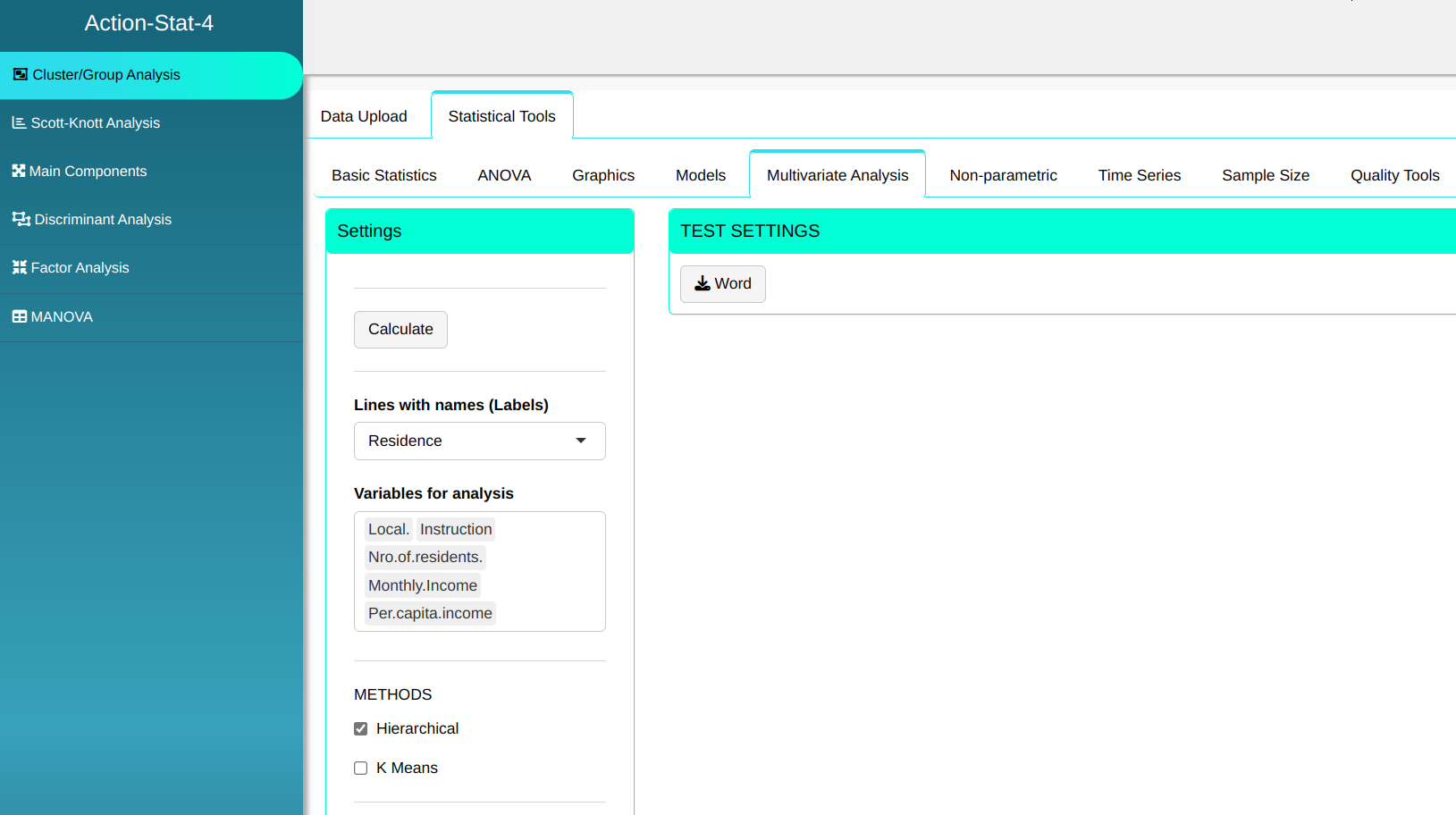
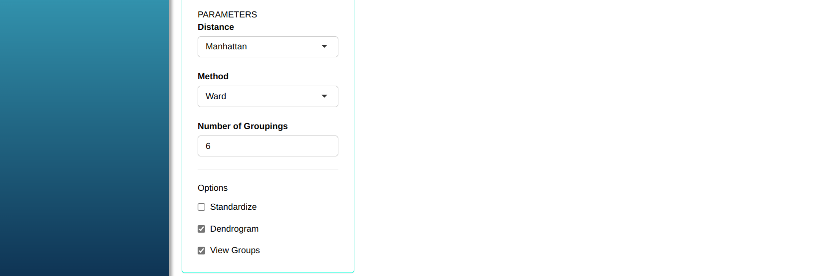
Then click Calculate to get the results. You can also generate the analyses and download them in Word format.
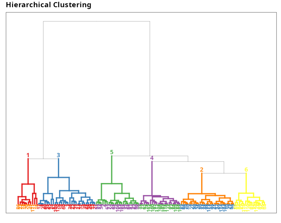
Hierarchical Clustering
| Group 1 | Group 2 | Group 3 | Group 4 | Group 5 | Group 6 |
|---|---|---|---|---|---|
| 1 | 2 | 4 | 6 | 24 | 35 |
| 3 | 11 | 10 | 7 | 44 | 43 |
| 5 | 13 | 19 | 32 | 73 | 45 |
| 8 | 15 | 21 | 34 | 77 | 46 |
| 9 | 18 | 26 | 37 | 78 | 62 |
| 12 | 20 | 29 | 42 | 82 | 64 |
| 14 | 22 | 30 | 50 | 84 | 67 |
| 16 | 47 | 33 | 52 | 88 | 87 |
| 17 | 86 | 38 | 53 | 90 | 89 |
| 23 | 111 | 41 | 58 | 92 | 95 |
| 25 | 51 | 61 | 97 | 96 | |
| 27 | 54 | 63 | 100 | 110 | |
| 28 | 57 | 68 | 102 | 115 | |
| 31 | 59 | 72 | 103 | 116 | |
| 36 | 66 | 75 | 105 | 117 | |
| 39 | 69 | 76 | 107 | ||
| 40 | 70 | 83 | 108 | ||
| 48 | 79 | 91 | 112 | ||
| 49 | 80 | 94 | 118 | ||
| 55 | 85 | 101 | 119 | ||
| 56 | 93 | 106 | |||
| 60 | 98 | ||||
| 65 | 99 | ||||
| 71 | 104 | ||||
| 74 | 113 | ||||
| 81 | 114 | ||||
| 109 | |||||
| 120 |
Group
| Labels | Residual Order | Groups |
|---|---|---|
| 1 | 1 | 1 |
| 2 | 2 | 2 |
| 3 | 3 | 1 |
| 4 | 4 | 3 |
| 5 | 5 | 1 |
| 6 | 6 | 4 |
| 7 | 7 | 4 |
| 8 | 8 | 1 |
| 9 | 9 | 1 |
| 10 | 10 | 3 |
| 11 | 11 | 2 |
| 12 | 12 | 1 |
| 13 | 13 | 2 |
| 14 | 14 | 1 |
| 15 | 15 | 2 |
| 16 | 16 | 1 |
| 17 | 17 | 1 |
| 18 | 18 | 2 |
| 19 | 19 | 3 |
| 20 | 20 | 2 |
| 21 | 21 | 3 |
| 22 | 22 | 2 |
| 23 | 23 | 1 |
| 24 | 24 | 5 |
| 25 | 25 | 1 |
| 26 | 26 | 3 |
| 27 | 27 | 1 |
| 28 | 28 | 1 |
| 29 | 29 | 3 |
| 30 | 30 | 3 |
| 31 | 31 | 1 |
| 32 | 32 | 4 |
| 33 | 33 | 3 |
| 34 | 34 | 4 |
| 35 | 35 | 6 |
| 36 | 36 | 1 |
| 37 | 37 | 4 |
| 38 | 38 | 3 |
| 39 | 39 | 1 |
| 40 | 40 | 1 |
| 41 | 41 | 3 |
| 42 | 42 | 4 |
| 43 | 43 | 6 |
| 44 | 44 | 5 |
| 45 | 45 | 6 |
| 46 | 46 | 6 |
| 47 | 47 | 2 |
| 48 | 48 | 1 |
| 49 | 49 | 1 |
| 50 | 50 | 4 |
| 51 | 51 | 3 |
| 52 | 52 | 4 |
| 53 | 53 | 4 |
| 54 | 54 | 3 |
| 55 | 55 | 1 |
| 56 | 56 | 1 |
| 57 | 57 | 3 |
| 58 | 58 | 4 |
| 59 | 59 | 3 |
| 60 | 60 | 1 |
| 61 | 61 | 4 |
| 62 | 62 | 6 |
| 63 | 63 | 4 |
| 64 | 64 | 6 |
| 65 | 65 | 1 |
| 66 | 66 | 3 |
| 67 | 67 | 6 |
| 68 | 68 | 4 |
| 69 | 69 | 3 |
| 70 | 70 | 3 |
| 71 | 71 | 1 |
| 72 | 72 | 4 |
| 73 | 73 | 5 |
| 74 | 74 | 1 |
| 75 | 75 | 4 |
| 76 | 76 | 4 |
| 77 | 77 | 5 |
| 78 | 78 | 5 |
| 79 | 79 | 3 |
| 80 | 80 | 3 |
| 81 | 81 | 1 |
| 82 | 82 | 5 |
| 83 | 83 | 4 |
| 84 | 84 | 5 |
| 85 | 85 | 3 |
| 86 | 86 | 2 |
| 87 | 87 | 6 |
| 88 | 88 | 5 |
| 89 | 89 | 6 |
| 90 | 90 | 5 |
| 91 | 91 | 4 |
| 92 | 92 | 5 |
| 93 | 93 | 3 |
| 94 | 94 | 4 |
| 95 | 95 | 6 |
| 96 | 96 | 6 |
| 97 | 97 | 5 |
| 98 | 98 | 3 |
| 99 | 99 | 3 |
| 100 | 100 | 5 |
| 101 | 101 | 4 |
| 102 | 102 | 5 |
| 103 | 103 | 5 |
| 104 | 104 | 3 |
| 105 | 105 | 5 |
| 106 | 106 | 4 |
| 107 | 107 | 5 |
| 108 | 108 | 5 |
| 109 | 109 | 1 |
| 110 | 110 | 6 |
| 111 | 111 | 2 |
| 112 | 112 | 5 |
| 113 | 113 | 3 |
| 114 | 114 | 3 |
| 115 | 115 | 6 |
| 116 | 116 | 6 |
| 117 | 117 | 6 |
| 118 | 118 | 5 |
| 119 | 119 | 5 |
| 120 | 120 | 1 |
Example 5:
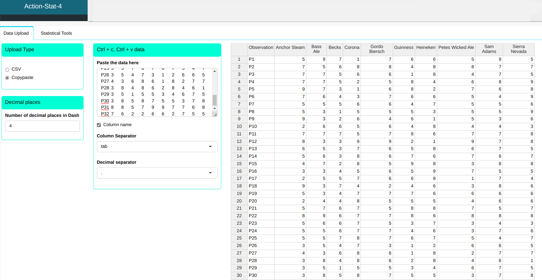
A brewery wants to study its customers' tastes in relation to certain brands of beer. The table below shows the results of a study of the perceptions and preferences of 32 students about 10 different brands of beer. Each student rated the 10 beer brands on a 10-point scale: Anchor Steam, Bass Ale, Beck's, Corona, Gordo-Biersch, Guinness, Heineken, Pete's Wicked Ale, Sam Adams, Sierra and Nevada. We will apply Cluster Analysis using the K-means method to compare the groups.
| Observation | Anchor Steam | Bass Ale | Beck's | Corona | Gordo-Biersch | Guinness | Heineken | Pete's Wicked Ale | Sam Adams | Sierra Nevada |
|---|---|---|---|---|---|---|---|---|---|---|
| P1 | 5 | 9 | 7 | 1 | 7 | 6 | 6 | 5 | 9 | 5 |
| P2 | 7 | 5 | 6 | 8 | 8 | 4 | 8 | 8 | 7 | 7 |
| P3 | 7 | 7 | 5 | 6 | 6 | 1 | 8 | 4 | 7 | 5 |
| P4 | 7 | 7 | 5 | 2 | 5 | 8 | 4 | 6 | 8 | 9 |
| P5 | 9 | 7 | 3 | 1 | 6 | 8 | 2 | 7 | 6 | 8 |
| P6 | 7 | 6 | 4 | 3 | 7 | 6 | 6 | 5 | 4 | 9 |
| P7 | 5 | 5 | 5 | 6 | 6 | 4 | 7 | 5 | 5 | 6 |
| P8 | 5 | 3 | 1 | 5 | 5 | 5 | 3 | 5 | 5 | 9 |
| P9 | 9 | 3 | 2 | 6 | 4 | 6 | 1 | 5 | 3 | 6 |
| P10 | 2 | 6 | 6 | 5 | 6 | 4 | 8 | 4 | 4 | 3 |
| P11 | 7 | 7 | 7 | 5 | 7 | 8 | 6 | 7 | 7 | 8 |
| P12 | 8 | 3 | 3 | 9 | 9 | 2 | 1 | 9 | 7 | 8 |
| P13 | 6 | 5 | 3 | 7 | 6 | 5 | 8 | 6 | 7 | 5 |
| P14 | 5 | 6 | 3 | 8 | 6 | 7 | 6 | 7 | 6 | 7 |
| P15 | 4 | 7 | 2 | 8 | 5 | 9 | 8 | 3 | 8 | 8 |
| P16 | 3 | 3 | 4 | 5 | 6 | 5 | 9 | 7 | 5 | 5 |
| P17 | 2 | 5 | 5 | 7 | 6 | 6 | 8 | 1 | 7 | 4 |
| P18 | 9 | 3 | 7 | 4 | 2 | 4 | 6 | 3 | 8 | 6 |
| P19 | 5 | 3 | 4 | 7 | 7 | 7 | 6 | 6 | 6 | 6 |
| P20 | 2 | 4 | 4 | 8 | 5 | 5 | 5 | 4 | 6 | 6 |
| P21 | 5 | 7 | 6 | 7 | 5 | 8 | 8 | 7 | 5 | 7 |
| P22 | 8 | 9 | 6 | 7 | 7 | 8 | 6 | 8 | 8 | 8 |
| P23 | 5 | 6 | 6 | 7 | 5 | 3 | 7 | 3 | 4 | 3 |
| P24 | 5 | 5 | 6 | 7 | 7 | 4 | 6 | 3 | 7 | 6 |
| P25 | 5 | 5 | 7 | 8 | 7 | 6 | 7 | 5 | 4 | 7 |
| P26 | 3 | 5 | 4 | 7 | 3 | 1 | 2 | 6 | 6 | 5 |
| P27 | 4 | 3 | 6 | 8 | 6 | 1 | 8 | 2 | 7 | 7 |
| P28 | 3 | 8 | 4 | 8 | 6 | 2 | 8 | 4 | 6 | 1 |
| P29 | 3 | 5 | 1 | 5 | 5 | 3 | 4 | 6 | 7 | 5 |
| P30 | 3 | 8 | 5 | 8 | 7 | 5 | 5 | 3 | 7 | 8 |
| P31 | 8 | 8 | 5 | 7 | 9 | 9 | 7 | 7 | 6 | 8 |
| P32 | 7 | 6 | 2 | 2 | 6 | 6 | 2 | 7 | 5 | 5 |
We will upload the data to the system.
Configuring as shown in the figure below to perform the analysis of clustering.
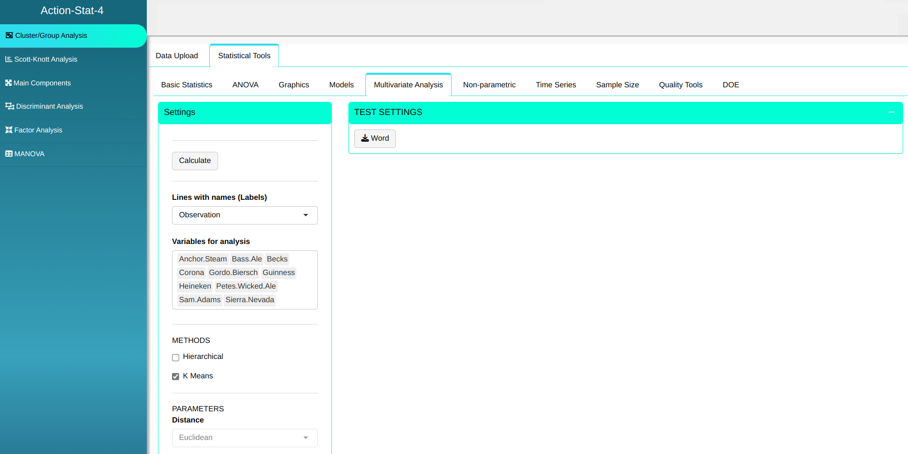

Then click Calculate to get the results. You can also generate the analyses and download them in Word format.
The results are:
K - Mean Clustering
| Group 1 | Group 2 |
|---|---|
| P1 | P3 |
| P2 | P7 |
| P4 | P10 |
| P5 | P13 |
| P6 | P16 |
| P8 | P17 |
| P9 | P18 |
| P11 | P20 |
| P12 | P23 |
| P14 | P24 |
| P15 | P25 |
| P19 | P26 |
| P21 | P27 |
| P22 | P28 |
| P31 | P29 |
| P32 | P30 |
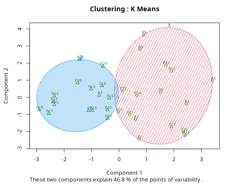
Note that the K-means method grouped the customers into 2 groups. We can put together a table with the average scores each group gave to the beer brands.
In Group 1, beers that were \“dark\” and had a \“stronger\” flavor had a higher mean. a higher mean; in Group 2, “light” colored beers had the highest mean. A possible conclusion from this segmentation is as follows:
Customers classified in Group 1 have a greater preference for dark dark beers with a more intense taste, while those classified in Group Group 2 have a greater preference for \“light\” colored beers.