1. ANOVA Fixed Effect
ANOVA is used to analyze the behavior of various treatments of a factor applied to the process and/or product.
Example 1:
Consider a process, product or service in which we want to evaluate the impact of factor A, such that A has k levels, these levels being fixed. Suppose that a sample of N experimental units is selected completely at random from a population of experimental units . The experimental unit is the basic unit to which the treatments are applied.
| Factor | Resistance |
|---|---|
| 15 | 7 |
| 15 | 7 |
| 15 | 15 |
| 15 | 11 |
| 15 | 9 |
| 20 | 12 |
| 20 | 17 |
| 20 | 12 |
| 20 | 18 |
| 20 | 18 |
| 25 | 14 |
| 25 | 18 |
| 25 | 18 |
| 25 | 19 |
| 25 | 19 |
| 30 | 19 |
| 30 | 25 |
| 30 | 22 |
| 30 | 19 |
| 30 | 23 |
| 35 | 7 |
| 35 | 10 |
| 35 | 11 |
| 35 | 15 |
| 35 | 11 |
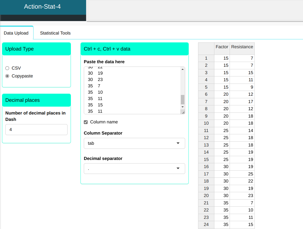
We will carry out a fixed-effect ANOVA
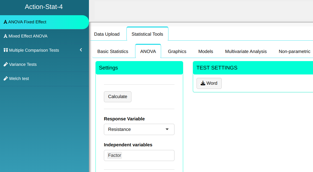
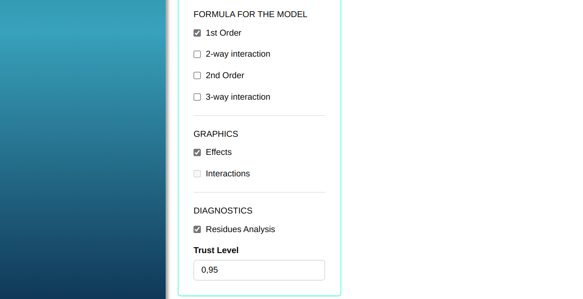
Then click Calculate to get the results. You can also generate the analyses and download them in Word format.

The results are:
ANOVA table
| D.F. | Sum of Squares | Mean Square | F Stat. | P-value | |
|---|---|---|---|---|---|
| Factor | 4 | 475.76 | 118.94 | 14.757 | 0 |
| Residuals | 20 | 161.20 | 8.06 |
Confidence Interval of the Effect Factor
| Level | Lower Limit | Mean Effect | Upper Limit |
|---|---|---|---|
| 15 | 7.152 | 9.8 | 12.448 |
| 20 | 12.752 | 15.4 | 18.048 |
| 25 | 14.952 | 17.6 | 20.248 |
| 30 | 18.952 | 21.6 | 24.248 |
| 35 | 8.152 | 10.8 | 13.448 |
Normality test
| Value | |
|---|---|
| Mean | 0.000 |
| Standard Deviation | 2.592 |
| N | 25.000 |
| Anderson-Darling | 0.519 |
| P-Value | 0.170 |
In this example, the Sum of Squares of the Factor (475.76) is much greater than the Sum of Squares of the Error (161.20), which already indicates that the mean are not equal.
If the P-value is less than or equal to the predetermined significance level ($\alpha$), this means that the means of the levels are different. Otherwise, they are equal. In this case, as it is less than 0.05, we reject the null hypothesis that these means are equal, i.e. we can say that the means of the levels are different.
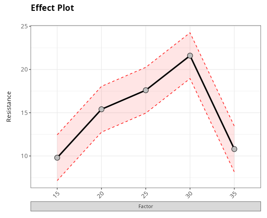
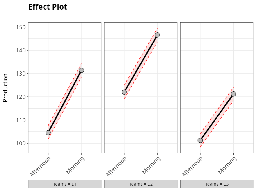
In the effects graph, the black dots are the mean of each factor level, which in the table are called Effects.
The red lines represent the confidence interval for the averages of the factor levels.
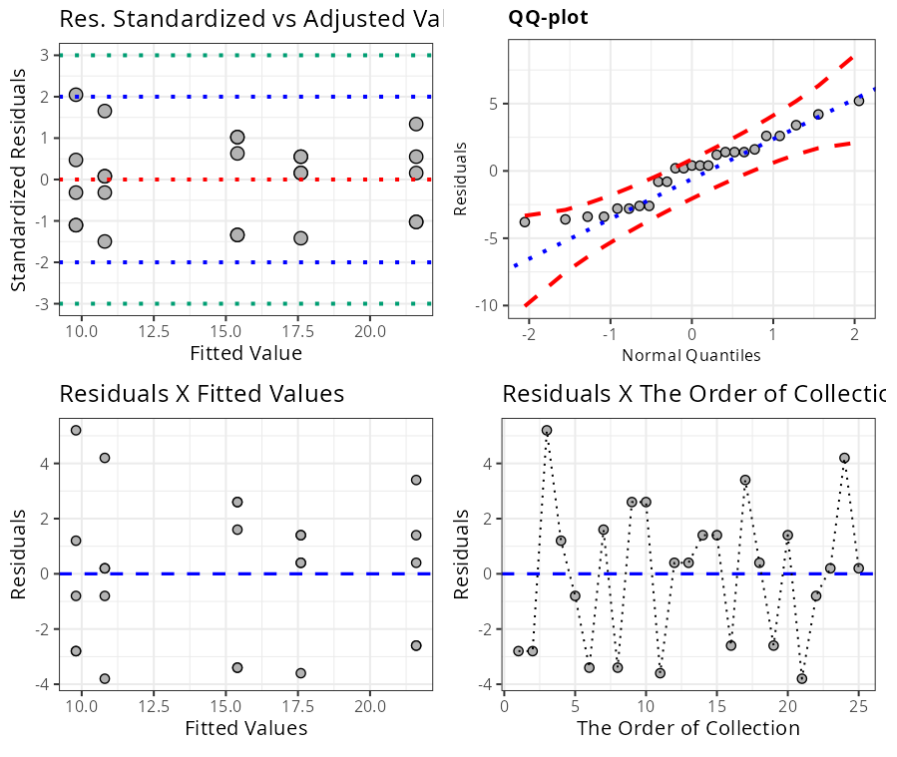
Graph 1: Graph of Standardized Residuals versus Fitted Values.
Graph 2: Graph of Residuals versus Quantiles of the Normal.
Graph 3: Graph of Residuals versus Adjusted Values.
Graph 4: Graph the Residuals versus Order of Collection graph to see if the residuals are independent. The criterion for the analysis is: if the points on the graph are randomly distributed, this indicates independence, while if they show a pattern, this indicates dependence in the residuals. In our case, we verified independence in the residuals.
In our case, we will use the Anderson-Darling test, where the null hypothesis is the normality of the data, and by example, we verify that we do not reject (\“accept\”) the null hypothesis and thus verify the normality of the residuals.
Example 2:
A company that produces windshield wipers for automobiles wants to know how the factors Type of Reduction Gearbox and Type of Shaft, used in the manufacture of the motors that drive the wipers, influence the noise produced when they are used. To do this, we conducted an experiment with 54 motors, with 3 types of Shaft (Rolled, Cut and Imported) and 2 types of Reduction Gearboxes (Domestic and Imported). For each motor (experimental unit) we measured the noise. The data are in the table.
| Axis | Reducer box | Noise |
|---|---|---|
| Rolled | Imported | 39.6 |
| Rolled | National | 42.1 |
| Imported | National | 40.9 |
| Cut | National | 38.2 |
| Rolled | National | 42 |
| Cut | Imported | 41.3 |
| Imported | Imported | 39.6 |
| Rolled | National | 40.3 |
| Imported | National | 40.7 |
| Imported | Imported | 36.9 |
| Rolled | Imported | 40.2 |
| Cut | Imported | 46.8 |
| Cut | Imported | 40.3 |
| Cut | National | 37.4 |
| Cut | National | 37 |
| Rolled | Imported | 48.4 |
| Imported | Imported | 39.9 |
| Imported | National | 39.4 |
| Rolled | Imported | 40.9 |
| Rolled | National | 38.9 |
| Cut | Imported | 40.5 |
| Cut | National | 42.3 |
| Imported | Imported | 38.1 |
| Imported | Imported | 38 |
| Imported | Imported | 36.2 |
| Rolled | Imported | 41 |
| Cut | Imported | 39.9 |
| Rolled | Imported | 41 |
| Cut | National | 41.3 |
| Imported | National | 42 |
| Cut | Imported | 39.3 |
| Cut | National | 42.1 |
| Imported | Imported | 36.7 |
| Cut | National | 40.5 |
| Rolled | National | 38.9 |
| Imported | Imported | 37.2 |
| Rolled | Imported | 39.9 |
| Rolled | National | 43.7 |
| Imported | National | 41.4 |
| Rolled | National | 41 |
| Cut | Imported | 41.3 |
| Imported | National | 41.3 |
| Imported | Imported | 36.7 |
| Rolled | National | 40.1 |
| Cut | National | 41.3 |
| Rolled | Imported | 41 |
| Imported | National | 40.6 |
| Cut | National | 40.4 |
| Rolled | National | 40.3 |
| Imported | National | 41.3 |
| Cut | Imported | 40.1 |
| Rolled | Imported | 42.7 |
| Cut | Imported | 41.6 |
| Imported | National | 41.6 |
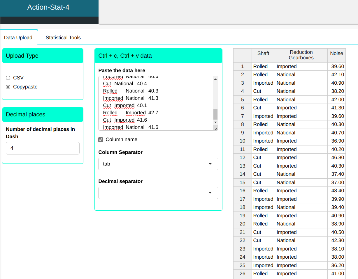
We will upload the data to the system.
We will carry out a fixed-effect ANOVA
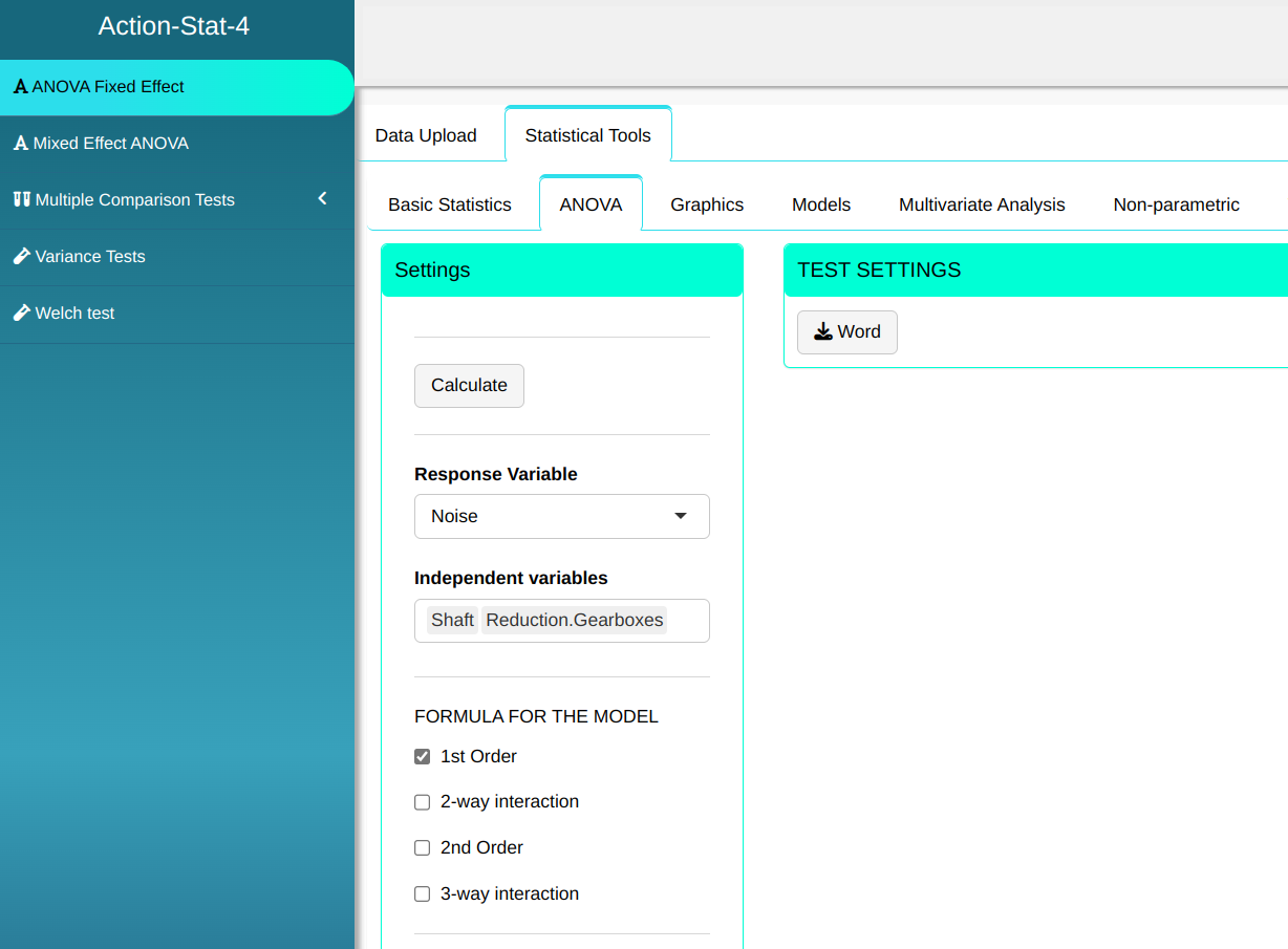

Then click Calculate to get the results. You can also generate the analyses and download them in Word format.
The results are:
ANOVA Table
| D.F. | Sum of Squares | Mean Squares | F Stat. | P-value | |
|---|---|---|---|---|---|
| Axis | 2 | 32.667 | 16.3335 | 4.6721 | 0.014 |
| Reducer box | 1 | 2.6224 | 2.6224 | 0.7501 | 0.3907 |
| Axis:Reducer box | 2 | 56.3293 | 28.1646 | 8.0563 | 0.001 |
| Residuals | 48 | 167.8067 | 3.496 |
Confidence Interval of the Effect Axis*Reducer box
| Level | Lower Limit | Mean Effect | Upper Limit |
|---|---|---|---|
| Cut/Imported | 39.9802 | 41.2333 | 42.4865 |
| Imported/Imported | 36.4469 | 37.7 | 38.9531 |
| Rolled/Imported | 40.3802 | 41.6333 | 42.8865 |
| Cut/National | 38.8024 | 40.0556 | 41.3087 |
| Imported/National | 39.7691 | 41.0222 | 42.2754 |
| Rolled/National | 39.558 | 40.8111 | 42.0642 |
Normality Test
| Value | |
|---|---|
| Mean | 0.000 |
| Standard Deviation | 1.7794 |
| N | 54 |
| Anderson-Darling | 1.2734 |
| P-Value | 0.0024 |
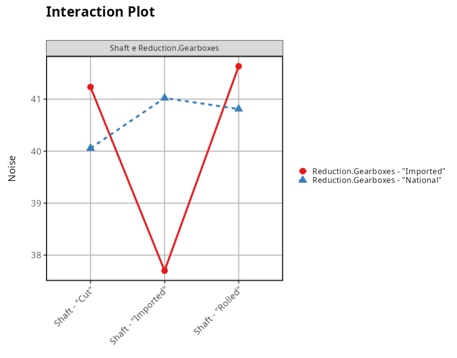
As the P-value associated with the interaction between the axle and the gearbox is very small (0.001), we conclude that the interaction between these factors is significant. We therefore have to be careful when interpreting the factors.
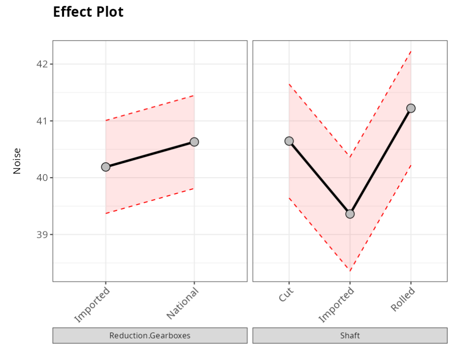
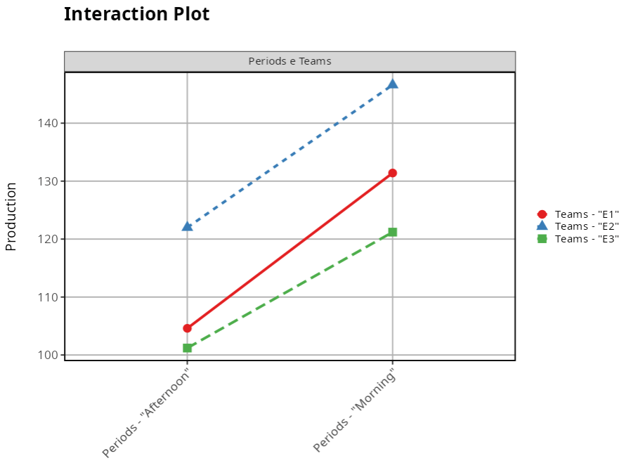
To assess whether there is an interaction, all we have to do is check whether the graphs of the factors intersect, as in the figure. We then conclude that there is interaction between the Gearbox and Axle factors.
In the graph, the black dots are the averages of each factor level, which in the table are called Effects. The red lines represent the confidence interval for the averages of the factor levels.
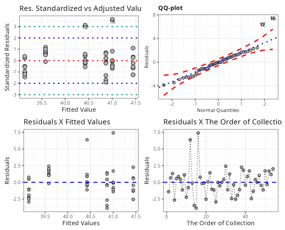
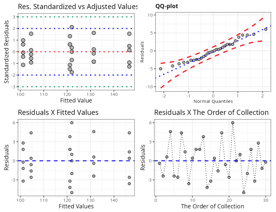
Graph 1: Graph of Standardized Residuals versus Fitted Values.
Graph 2: Graph of Residuals versus Quantiles of the Normal.
Graph 3: Graph of Residuals versus Adjusted Values.
Graph 4: Graph the Residuals versus Order of Collection graph to see if the residuals are independent. The criterion for the analysis is: if the points on the graph are randomly distributed, this indicates independence, while if they show a pattern, this indicates dependence in the residuals. In our case, we verified independence in the residuals.
In this case, we will use the Anderson-Darling test, where the null hypothesis is the normality of the data, and from the example, we see that we reject the null hypothesis and thus verify that the residuals do not follow a normal distribution.
Example 3
A company’s operations manager monitors the daily output of three fixed assembly teams (E1, E2, and E3) working extended shifts that cover both the Morning and Afternoon periods. It is suspected that accumulated physical fatigue causes a general drop in productivity during the afternoon shift and that the teams have different average production capacities. A sample covering five days of operation was collected for each team-period combination, recording the output (units produced per hour).
| Periods | Teams | Production |
|---|---|---|
| Morning | E1 | 131 |
| Morning | E1 | 129 |
| Morning | E1 | 132 |
| Morning | E1 | 136 |
| Morning | E1 | 129 |
| Morning | E2 | 144 |
| Morning | E2 | 151 |
| Morning | E2 | 148 |
| Morning | E2 | 143 |
| Morning | E2 | 147 |
| Morning | E3 | 123 |
| Morning | E3 | 123 |
| Morning | E3 | 125 |
| Morning | E3 | 117 |
| Morning | E3 | 118 |
| Afternoon | E1 | 105 |
| Afternoon | E1 | 103 |
| Afternoon | E1 | 109 |
| Afternoon | E1 | 104 |
| Afternoon | E1 | 102 |
| Afternoon | E2 | 128 |
| Afternoon | E2 | 122 |
| Afternoon | E2 | 123 |
| Afternoon | E2 | 117 |
| Afternoon | E2 | 120 |
| Afternoon | E3 | 103 |
| Afternoon | E3 | 98 |
| Afternoon | E3 | 104 |
| Afternoon | E3 | 100 |
| Afternoon | E3 | 101 |
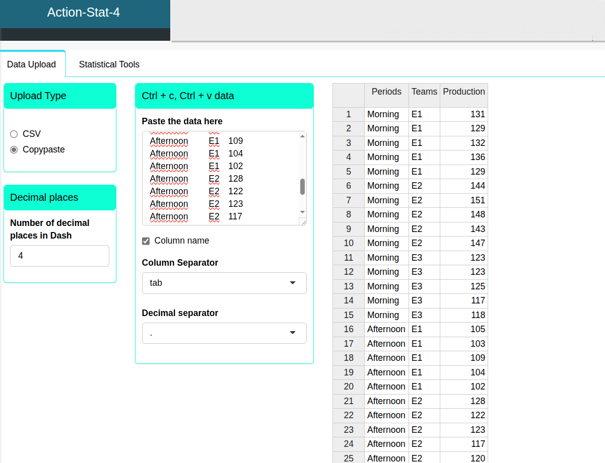
We will upload the data to the system.
We will carry out a fixed-effect ANOVA
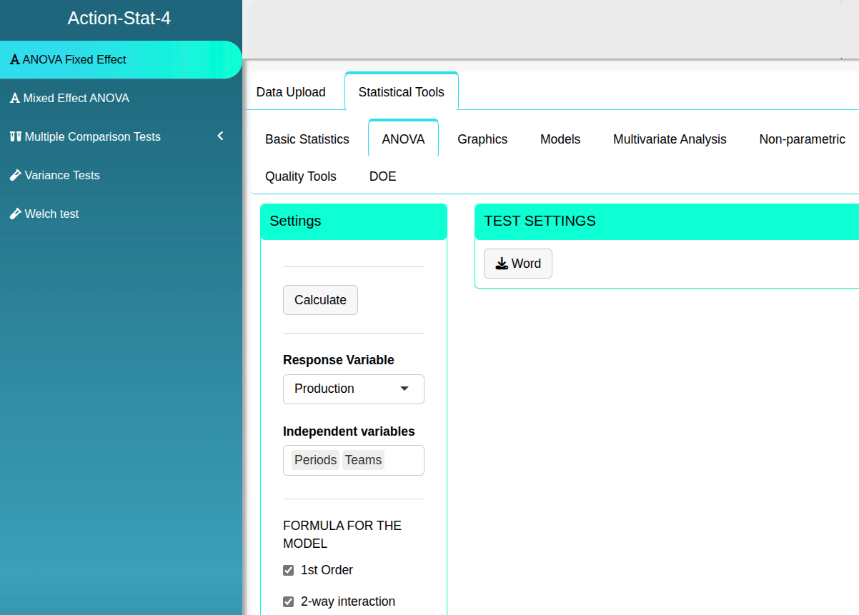

Then click Calculate to get the results. You can also generate the analyses and download them in Word format.
The results are:
ANOVA table
| D.F. | Sum of Square | Mean Square | F. Stat. | P-value | |
|---|---|---|---|---|---|
| Periods | 2 | $\qquad$4248.3 | $\qquad$4248.3 | 422.7164 | 0 |
| Teams | 1 | $\qquad$2818.4667 | $\qquad$1409.2333 | 140.2222 | 0 |
| Periods:Teams | 2 | $\qquad$60.2 | $\qquad$30.1 | 2.995 | 0.069 |
| Residual | 24 | $\qquad$241.2 | $\qquad$10.05 |
Confidence Interval of the Effect Periods*Teams
| Level | Lower Limit | Mean Effect | Upper Limit |
|---|---|---|---|
| Afternoon/E1 | $\quad$101.6739 | $\qquad$104.6 | $\quad$107.5261 |
| Morning/E1 | $\quad$128.4739 | $\qquad$131.4 | $\quad$134.3261 |
| Afternoon/E2 | $\quad$119.0739 | $\qquad$122 | $\quad$124.9261 |
| Morning/E2 | $\quad$143.6739 | $\qquad$146.6 | $\quad$149.5261 |
| Afternoon/E3 | $\quad$98.2739 | $\qquad$101.2 | $\quad$104.1261 |
| Morning/E3 | $\quad$118.2739 | $\qquad$121.2 | $\quad$124.1261 |
Normality tests
| Value | |
|---|---|
| Mean | 0 |
| Standard Deviation | 2.884 |
| N | 30 |
| Anderson-Darling | 0.287 |
| P-Value | 0.5975 |