4. Discriminant Analysis
Discriminant analysis is a statistical technique used to classifying elements of a sample or population. It requires priori knowledge of the characteristics of the elements in the sample (or population). This knowledge is used to classify new elements into existing groups. In this method, the number of groups must be known a priori.
Example 1:
The table below contains data from 21 companies, collected approximately 2 years before they went bankrupt and another 25 companies that did not go bankrupt in the period.
| Company | Group | Cash flow | Company income | Current equity | Income from sales |
|---|---|---|---|---|---|
| 1 | 1 | -0.45 | -0.41 | 1.09 | 0.45 |
| 2 | 1 | -0.56 | -0.31 | 1.51 | 0.16 |
| 3 | 1 | 0.06 | 0.02 | 1.01 | 0.4 |
| 4 | 1 | -0.07 | -0.09 | 1.45 | 0.26 |
| 5 | 1 | -0.1 | -0.09 | 1.56 | 0.67 |
| 6 | 1 | -0.14 | -0.07 | 0.71 | 0.28 |
| 7 | 1 | 0.04 | 0.01 | 1.5 | 0.71 |
| 8 | 1 | -0.07 | -0.06 | 1.37 | 0.4 |
| 9 | 1 | 0.07 | -0.01 | 1.37 | 0.34 |
| 10 | 1 | -0.14 | -0.14 | 1.42 | 0.43 |
| 11 | 1 | -0.23 | -0.3 | 0.33 | 0.18 |
| 12 | 1 | 0.07 | 0.02 | 1.31 | 0.25 |
| 13 | 1 | 0.01 | 0 | 2.15 | 0.7 |
| 14 | 1 | -0.28 | -0.23 | 1.19 | 0.66 |
| 15 | 1 | 0.15 | 0.05 | 1.88 | 0.27 |
| 16 | 1 | 0.37 | 0.11 | 1.99 | 0.38 |
| 17 | 1 | -0.08 | -0.08 | 1.51 | 0.42 |
| 18 | 1 | 0.05 | 0.03 | 1.68 | 0.95 |
| 19 | 1 | 0.01 | 0 | 1.26 | 0.6 |
| 20 | 1 | 0.12 | 0.11 | 1.14 | 0.17 |
| 21 | 1 | -0.28 | -0.29 | 1.27 | 0.51 |
| 22 | 2 | 0.51 | 0.1 | 2.49 | 0.54 |
| 23 | 2 | 0.08 | 0.02 | 2.01 | 0.53 |
| 24 | 2 | 0.38 | 0.11 | 3.27 | 0.35 |
| 25 | 2 | 0.19 | 0.05 | 2.25 | 0.33 |
| 26 | 2 | 0.32 | 0.07 | 4.24 | 0.63 |
| 27 | 2 | 0.31 | 0.05 | 4.45 | 0.69 |
| 28 | 2 | 0.12 | 0.05 | 2.52 | 0.69 |
| 29 | 2 | -0.02 | 0.02 | 2.05 | 0.35 |
| 30 | 2 | 0.22 | 0.08 | 2.35 | 0.4 |
| 31 | 2 | 0.17 | 0.07 | 1.8 | 0.52 |
| 32 | 2 | 0.15 | 0.05 | 2.17 | 0.55 |
| 33 | 2 | -0.1 | -0.01 | 2.5 | 0.58 |
| 34 | 2 | 0.14 | -0.03 | 0.46 | 0.26 |
| 35 | 2 | 0.14 | 0.07 | 2.61 | 0.52 |
| 36 | 2 | 0.15 | 0.06 | 2.23 | 0.56 |
| 37 | 2 | 0.16 | 0.05 | 2.31 | 0.2 |
| 38 | 2 | 0.29 | 0.06 | 1.84 | 0.38 |
| 39 | 2 | 0.54 | 0.11 | 2.33 | 0.48 |
| 40 | 2 | -0.33 | -0.09 | 3.01 | 0.47 |
| 41 | 2 | 0.48 | 0.09 | 1.24 | 0.18 |
| 42 | 2 | 0.56 | 0.11 | 4.29 | 0.44 |
| 43 | 2 | 0.2 | 0.08 | 1.99 | 0.3 |
| 44 | 2 | 0.47 | 0.14 | 2.92 | 0.45 |
| 45 | 2 | 0.17 | 0.04 | 2.45 | 0.14 |
| 46 | 2 | 0.58 | 0.04 | 5.06 | 0.13 |
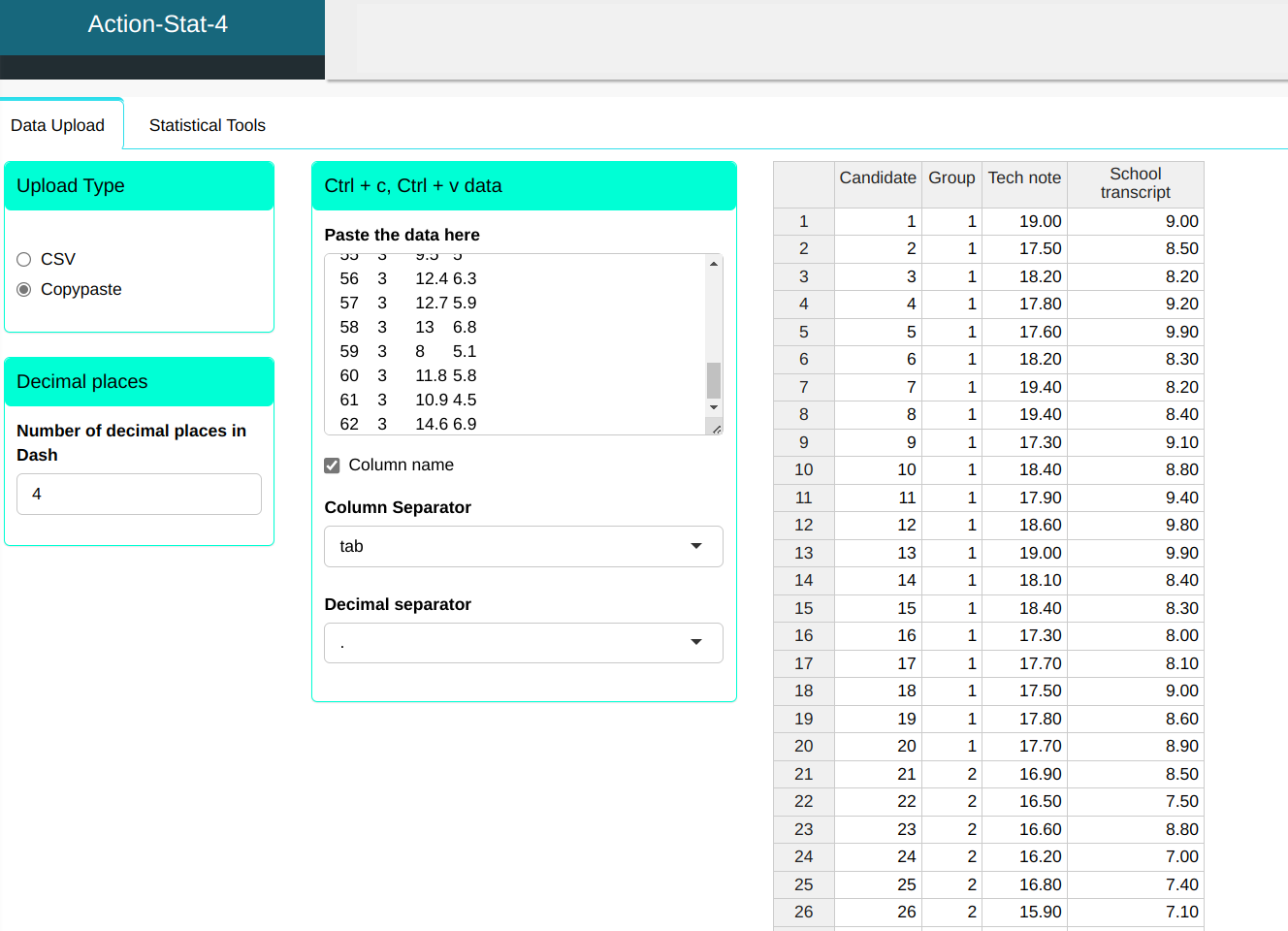
We will upload the data to the system.
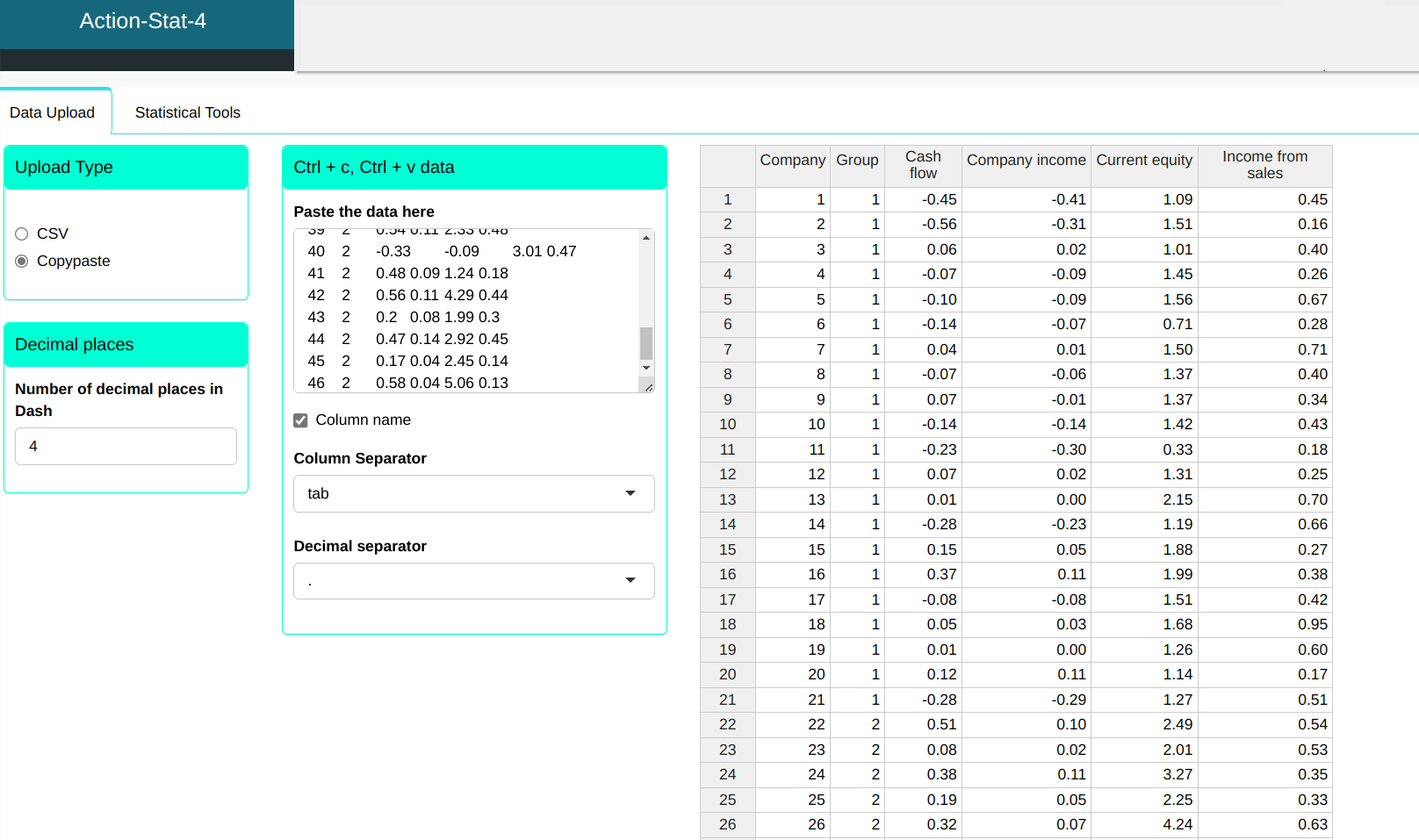
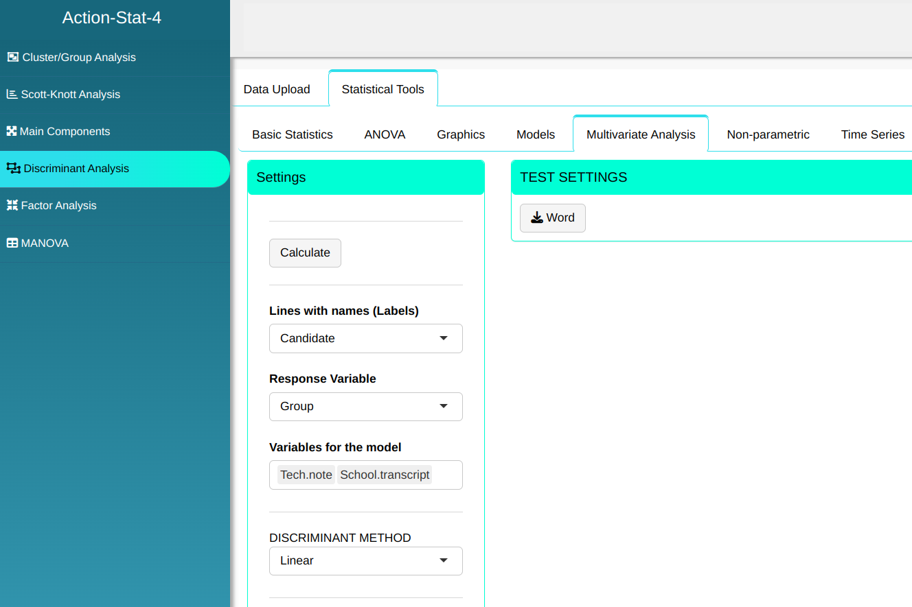
Configuring as shown in the figure below to perform the Discriminant analysis.


Then click Calculate to get the results. You can also generate the analyses and download them in Word format.

Os resultados são:
The Results of analysis
| 1 | 2 | |
|---|---|---|
| 1 | 19.00 | 2.000 |
| 2 | 1.00 | 24.000 |
| Total | 20.00 | 26.000 |
| Correct | 19.00 | 24.000 |
| Proportion: Correct | 0.95 | 0.923 |
Scores Table
| 1 | 2 | Classification | |
|---|---|---|---|
| 1 | 7.687 | 2.363 | 1 |
| 2 | 2.619 | -0.669 | 1 |
| 3 | 1.215 | 0.068 | 1 |
| 4 | 1.697 | 0.531 | 1 |
| 5 | 6.738 | 4.805 | 1 |
| 6 | 0.108 | -2.278 | 1 |
| 7 | 5.876 | 4.758 | 1 |
| 8 | 2.729 | 1.362 | 1 |
| 9 | 1.648 | 1.009 | 1 |
| 10 | 4.338 | 2.240 | 1 |
| 11 | 2.059 | -2.757 | 1 |
| 12 | -0.081 | -0.375 | 1 |
| 13 | 6.870 | 6.751 | 1 |
| 14 | 7.830 | 3.908 | 1 |
| 15 | 0.858 | 1.834 | 2 |
| 16 | 2.154 | 3.849 | 2 |
| 17 | 3.519 | 2.167 | 1 |
| 18 | 8.762 | 7.591 | 1 |
| 19 | 4.214 | 2.814 | 1 |
| 20 | -2.750 | -2.347 | 2 |
| 21 | 7.215 | 3.269 | 1 |
| 22 | 5.633 | 7.915 | 2 |
| 23 | 4.493 | 4.771 | 2 |
| 24 | 3.902 | 7.838 | 2 |
| 25 | 2.343 | 3.861 | 2 |
| 26 | 9.359 | 13.902 | 2 |
| 27 | 10.748 | 15.335 | 2 |
| 28 | 6.880 | 7.961 | 2 |
| 29 | 1.981 | 2.598 | 2 |
| 30 | 2.933 | 4.750 | 2 |
| 31 | 3.484 | 3.958 | 2 |
| 32 | 4.729 | 5.570 | 2 |
| 33 | 5.730 | 6.244 | 2 |
| 34 | -0.165 | -2.237 | 1 |
| 35 | 4.679 | 6.482 | 2 |
| 36 | 4.768 | 5.771 | 2 |
| 37 | 0.744 | 2.614 | 2 |
| 38 | 2.497 | 3.423 | 2 |
| 39 | 4.583 | 6.849 | 2 |
| 40 | 5.760 | 6.423 | 2 |
| 41 | -0.702 | 0.150 | 2 |
| 42 | 7.351 | 13.042 | 2 |
| 43 | 1.057 | 2.463 | 2 |
| 44 | 4.362 | 7.848 | 2 |
| 45 | 0.461 | 2.632 | 2 |
| 46 | 6.169 | 13.300 | 2 |
General Information
| Levels | Number of groups | Validation Type | Correct Total Porcentage | Erro Rate |
|---|---|---|---|---|
| 1 | 21 | Validation by learning dta | 31.4159665046225 % | 6.52173913043478 % |
| 2 | 25 |
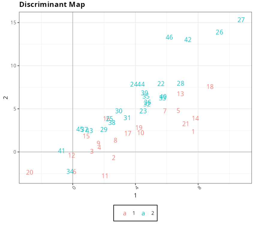
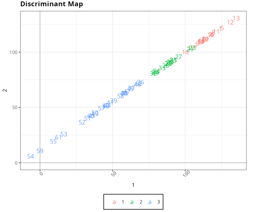
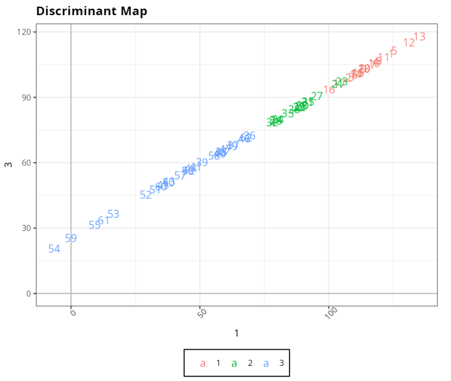
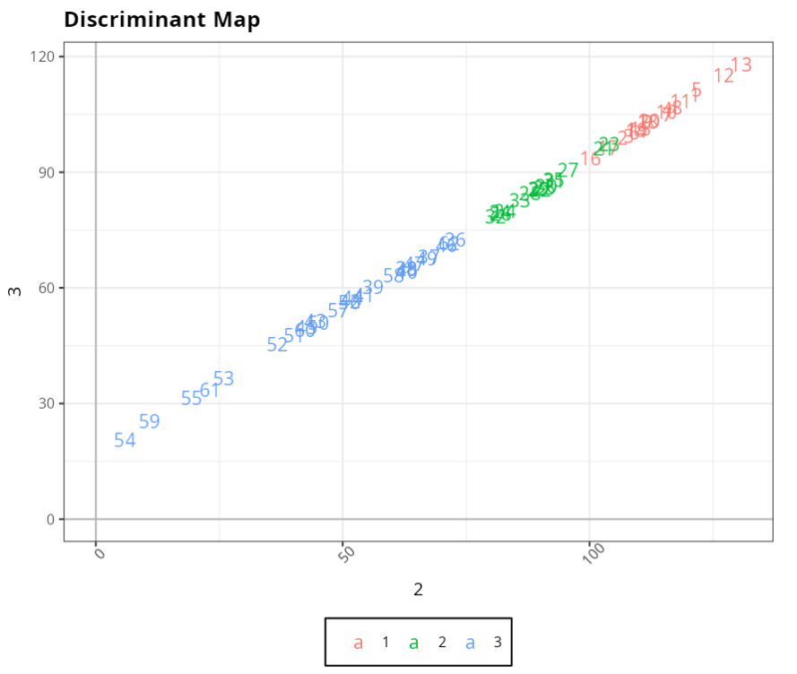
Example 2:
A postgraduate program wants to change the method of selecting its students to a technical students to a technical knowledge test and a grade assigned to the applicant’s applicant’s academic record. To do this, the 63 applicants from the previous year previous year were divided into three groups; (1) made up of the candidates (2) unsuccessful candidates, but who remained on the waiting list and (3) made up of candidates not approved for the program. The aim of the study is to verify whether the new selection method is able to discriminate well between candidates.
The data for this example is shown in the table below
| Candidate | Group | Tech note | School Transcript |
|---|---|---|---|
| 1 | 1 | 19 | 9 |
| 2 | 1 | 17.5 | 8.5 |
| 3 | 1 | 18.2 | 8.2 |
| 4 | 1 | 17.8 | 9.2 |
| 5 | 1 | 17.6 | 9.9 |
| 6 | 1 | 18.2 | 8.3 |
| 7 | 1 | 19.4 | 8.2 |
| 8 | 1 | 19.4 | 8.4 |
| 9 | 1 | 17.3 | 9.1 |
| 10 | 1 | 18.4 | 8.8 |
| 11 | 1 | 17.9 | 9.4 |
| 12 | 1 | 18.6 | 9.8 |
| 13 | 1 | 19 | 9.9 |
| 14 | 1 | 18.1 | 8.4 |
| 15 | 1 | 18.4 | 8.3 |
| 16 | 1 | 17.3 | 8 |
| 17 | 1 | 17.7 | 8.1 |
| 18 | 1 | 17.5 | 9 |
| 19 | 1 | 17.8 | 8.6 |
| 20 | 1 | 17.7 | 8.9 |
| 21 | 2 | 16.9 | 8.5 |
| 22 | 2 | 16.5 | 7.5 |
| 23 | 2 | 16.6 | 8.8 |
| 24 | 2 | 16.2 | 7 |
| 25 | 2 | 16.8 | 7.4 |
| 26 | 2 | 15.9 | 7.1 |
| 27 | 2 | 16.1 | 8.3 |
| 28 | 2 | 15.7 | 7.8 |
| 29 | 2 | 15.8 | 7.9 |
| 30 | 2 | 16.7 | 7.5 |
| 31 | 2 | 16.8 | 7.6 |
| 32 | 2 | 15.9 | 7 |
| 33 | 2 | 15.7 | 7.6 |
| 34 | 2 | 15.4 | 7.4 |
| 35 | 2 | 16.3 | 7.9 |
| 36 | 3 | 14.8 | 6.9 |
| 37 | 3 | 14.6 | 6.5 |
| 38 | 3 | 13.4 | 6.8 |
| 39 | 3 | 12.5 | 6.7 |
| 40 | 3 | 14.7 | 6 |
| 41 | 3 | 13.2 | 6.1 |
| 42 | 3 | 12.1 | 6.5 |
| 43 | 3 | 11 | 6.5 |
| 44 | 3 | 11.7 | 6.8 |
| 45 | 3 | 11.2 | 6.2 |
| 46 | 3 | 14.5 | 6.9 |
| 47 | 3 | 13.8 | 6.7 |
| 48 | 3 | 13.9 | 6.5 |
| 49 | 3 | 14.7 | 6.4 |
| 50 | 3 | 12.4 | 5.7 |
| 51 | 3 | 11.3 | 5.9 |
| 52 | 3 | 10.6 | 6 |
| 53 | 3 | 10.2 | 5.2 |
| 54 | 3 | 9 | 4 |
| 55 | 3 | 9.5 | 5 |
| 56 | 3 | 12.4 | 6.3 |
| 57 | 3 | 12.7 | 5.9 |
| 58 | 3 | 13 | 6.8 |
| 59 | 3 | 8 | 5.1 |
| 60 | 3 | 11.8 | 5.8 |
| 61 | 3 | 10.9 | 4.5 |
| 62 | 3 | 14.6 | 6.9 |
We will upload the data to the system.
Configuring as shown in the figure below to perform the Discriminant analysis.


Then click Calculate to get the results. You can also generate the analyses and download them in Word format.
Os resultados são:
The Results of analysis
| 1 | 2 | 3 | |
|---|---|---|---|
| constant | -118.000 | -92.924 | -55.731 |
| Tech.Note | 6.958 | 6.388 | 4.612 |
| School.transcript | 12.218 | 10.329 | 8.695 |
The Results of analysis
| 1 | 2 | 3 | |
|---|---|---|---|
| 1 | 19.000 | 1.000 | 0 |
| 2 | 2.000 | 13.000 | 0 |
| 3 | 0.000 | 2.000 | 25 |
| Total | 21.000 | 16.000 | 25 |
| Correct | 19.000 | 13.000 | 25 |
| Proportion: Correct | 0.905 | 0.812 | 1 |
Scores table
| 1 | 2 | 3 | Classification | |
|---|---|---|---|---|
| 1 | 124.165 | 121.411 | 110.146 | 1 |
| 2 | 107.619 | 106.664 | 98.881 | 1 |
| 3 | 108.824 | 108.037 | 99.5 | 1 |
| 4 | 118.259 | 115.811 | 106.351 | 1 |
| 5 | 125.42 | 121.763 | 111.515 | 1 |
| 6 | 110.046 | 109.07 | 100.37 | 1 |
| 7 | 117.173 | 115.703 | 105.034 | 1 |
| 8 | 119.617 | 117.768 | 106.773 | 1 |
| 9 | 113.558 | 111.584 | 103.176 | 1 |
| 10 | 117.546 | 115.512 | 105.64 | 1 |
| 11 | 121.399 | 118.515 | 108.551 | 1 |
| 12 | 131.156 | 127.118 | 115.257 | 1 |
| 13 | 135.161 | 130.707 | 117.972 | 1 |
| 14 | 110.572 | 109.464 | 100.778 | 1 |
| 15 | 111.437 | 110.347 | 101.292 | 1 |
| 16 | 100.118 | 100.222 | 93.611 | 2 |
| 17 | 104.123 | 103.81 | 96.325 | 1 |
| 18 | 113.728 | 111.828 | 103.229 | 1 |
| 19 | 110.928 | 109.613 | 101.134 | 1 |
| 20 | 113.898 | 112.073 | 103.281 | 1 |
| 21 | 103.444 | 102.831 | 96.114 | 1 |
| 22 | 88.443 | 89.947 | 85.574 | 2 |
| 23 | 105.022 | 104.013 | 97.339 | 1 |
| 24 | 80.246 | 82.866 | 79.843 | 2 |
| 25 | 89.308 | 90.83 | 86.088 | 2 |
| 26 | 79.38 | 81.982 | 79.329 | 2 |
| 27 | 95.434 | 95.655 | 90.686 | 2 |
| 28 | 86.542 | 87.935 | 84.493 | 2 |
| 29 | 88.459 | 89.607 | 85.824 | 2 |
| 30 | 89.834 | 91.224 | 86.496 | 2 |
| 31 | 91.752 | 92.896 | 87.827 | 2 |
| 32 | 78.159 | 80.949 | 78.46 | 2 |
| 33 | 84.098 | 85.869 | 82.754 | 2 |
| 34 | 79.567 | 81.887 | 79.632 | 2 |
| 35 | 91.938 | 92.801 | 88.13 | 2 |
| 36 | 69.283 | 72.89 | 72.517 | 2 |
| 37 | 63.004 | 67.48 | 68.117 | 3 |
| 38 | 58.32 | 62.913 | 65.192 | 3 |
| 39 | 50.836 | 56.131 | 60.172 | 3 |
| 40 | 57.591 | 62.955 | 64.23 | 3 |
| 41 | 48.376 | 54.405 | 58.183 | 3 |
| 42 | 45.61 | 51.51 | 56.588 | 3 |
| 43 | 37.956 | 44.483 | 51.515 | 3 |
| 44 | 46.492 | 52.054 | 57.352 | 3 |
| 45 | 35.682 | 42.662 | 49.829 | 3 |
| 46 | 67.196 | 70.973 | 71.134 | 3 |
| 47 | 59.882 | 64.436 | 66.167 | 3 |
| 48 | 58.134 | 63.009 | 64.889 | 3 |
| 49 | 62.478 | 67.086 | 67.708 | 3 |
| 50 | 37.922 | 45.163 | 51.015 | 3 |
| 51 | 32.712 | 40.202 | 47.682 | 3 |
| 52 | 29.064 | 36.763 | 45.323 | 3 |
| 53 | 16.506 | 25.945 | 36.522 | 3 |
| 54 | -6.506 | 5.885 | 20.554 | 3 |
| 55 | 9.192 | 19.408 | 31.555 | 3 |
| 56 | 45.253 | 51.361 | 56.232 | 3 |
| 57 | 42.453 | 49.146 | 54.138 | 3 |
| 58 | 55.537 | 60.358 | 63.347 | 3 |
| 59 | -0.023 | 10.858 | 25.507 | 3 |
| 60 | 34.969 | 42.363 | 49.118 | 3 |
| 61 | 12.823 | 23.186 | 33.664 | 3 |
| 62 | 67.892 | 71.612 | 71.595 | 2 |
General Information
| Levels | Nº of groups | Validation Type | Correct total Porcentage | Error rate |
|---|---|---|---|---|
| 1 | 20 | Validation by learning data | 31.0259359458277% | 8.06451612903226% |
| 2 | 15 | |||
| 3 | 27 |