3. Main Components
Principal component analysis is a method used to reduce the size of the problem into uncorrelated components which are linear combinations of the original variables. The number of these components is less than or equal to the number of original variables. This method is useful when the number of variables under study is very large.
The Action Principal Components tool allows you to reduce the dimension of the data through components which are linear combinations of the original variables.
Example 1:
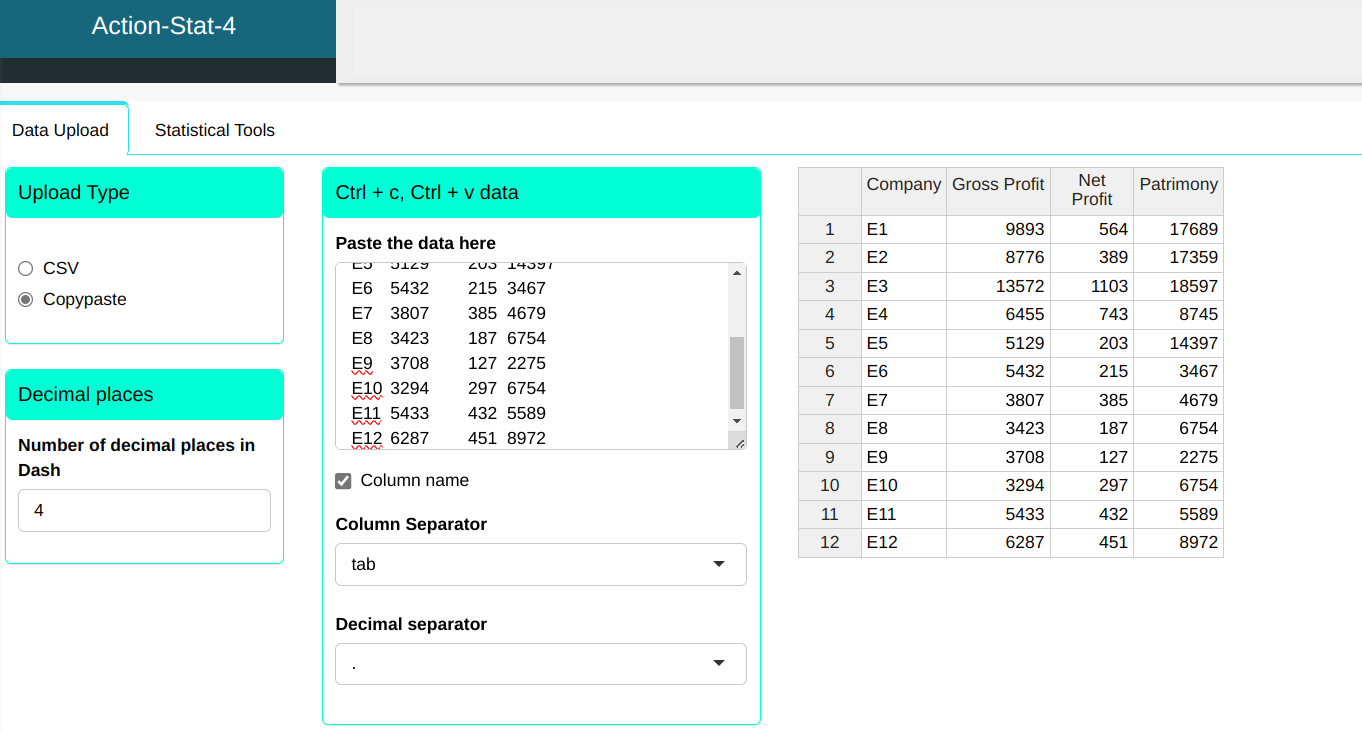
The table represents the gross profit, net profit and Patrimony, measured in monetary units, of 12 companies
| Company | Gross profit | Net Profit | Patrimony |
|---|---|---|---|
| E1 | 9893 | 564 | 17689 |
| E2 | 8776 | 389 | 17359 |
| E3 | 13572 | 1103 | 18597 |
| E4 | 6455 | 743 | 8745 |
| E5 | 5129 | 203 | 14397 |
| E6 | 5432 | 215 | 3467 |
| E7 | 3807 | 385 | 4679 |
| E8 | 3423 | 187 | 6754 |
| E9 | 3708 | 127 | 2275 |
| E10 | 3294 | 297 | 6754 |
| E11 | 5433 | 432 | 5589 |
| E12 | 6287 | 451 | 8972 |
Configuring as shown in the figure below to perform the main component analysis.
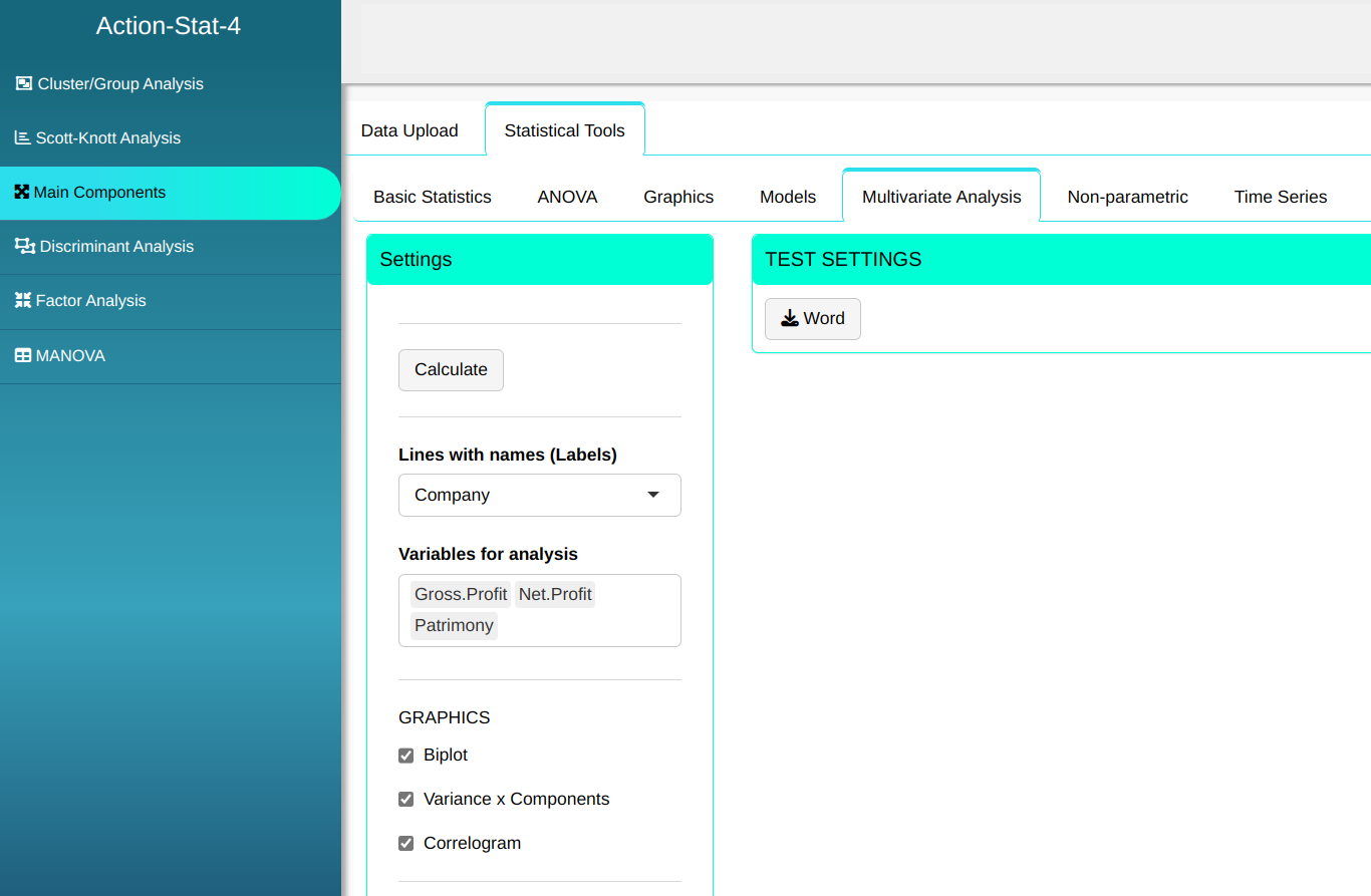

Then click Calculate to get the results. You can also generate the analyses and download them in Word format.

The results are:
Importance of the components
| Information | Comp.1 | Comp.2 | Comp.3 |
|---|---|---|---|
| Standard Deviation | 6165.889 | 1525.740 | 139.05 |
| Variance Proportion | 0.942 | 0.058 | 0.00 |
| Accumulated Proportion | 0.942 | 1.000 | 1.00 |
Table of component center
| Central Value | |
|---|---|
| Gross.Profit | 6267.417 |
| Net.Profit | 424.667 |
| Patrimony | 9606.417 |
Correlation Matrix
| Comp.1 | Comp.2 | Comp.3 | |
|---|---|---|---|
| Comp.1 | 1 | 0 | 0 |
| Comp.2 | 0 | 1 | 0 |
| Comp.3 | 0 | 0 | 1 |
Analysis Results
| Comp.1 | Comp.2 | Comp.3 | |
|---|---|---|---|
| Gross.Profit | 0.425 | 0.900 | 0.099 |
| Net.Profit | 0.028 | 0.097 | -0.995 |
| Patrimony | 0.905 | -0.426 | -0.016 |
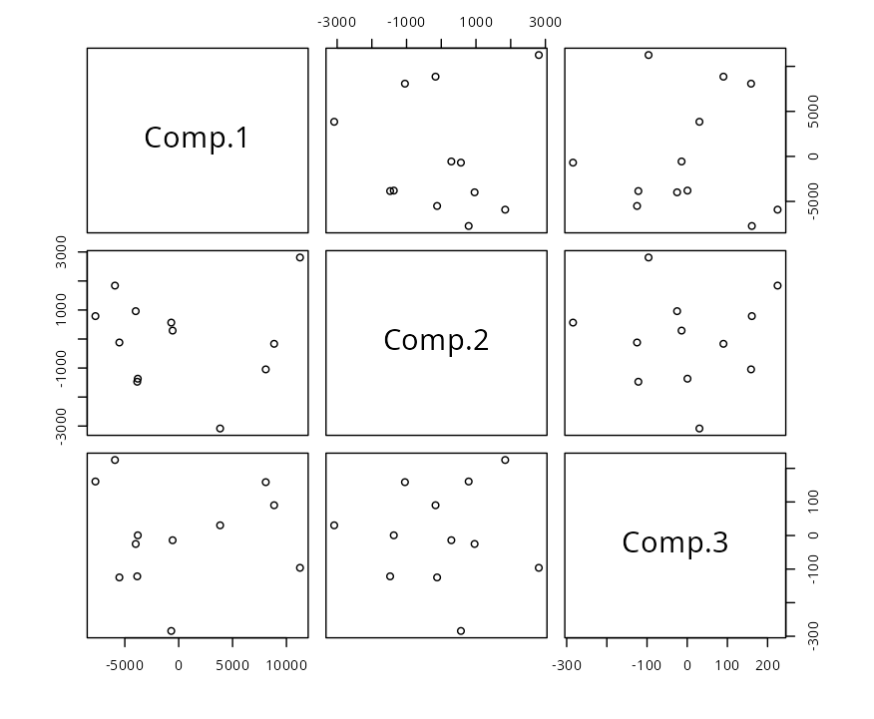
Analysis Results
| Comp.1 | Comp.2 | Comp.3 | |
|---|---|---|---|
| E1 | 8857.594 | -165.267 | 90.180 |
| E2 | 8079.361 | -1046.652 | 158.932 |
| E3 | 11257.926 | 2810.250 | -96.180 |
| E4 | -690.799 | 566.191 | -284.231 |
| E5 | 3844.091 | -3084.941 | 30.403 |
| E6 | -5915.416 | 1841.624 | 224.925 |
| E7 | -5504.970 | -119.929 | -124.811 |
| E8 | -3796.380 | -1367.834 | 0.640 |
| E9 | -7729.150 | 789.459 | 160.881 |
| E10 | -3848.175 | -1473.279 | -121.587 |
| E11 | -3989.162 | 960.153 | -25.133 |
| E12 | -564.919 | 290.226 | -14.019 |
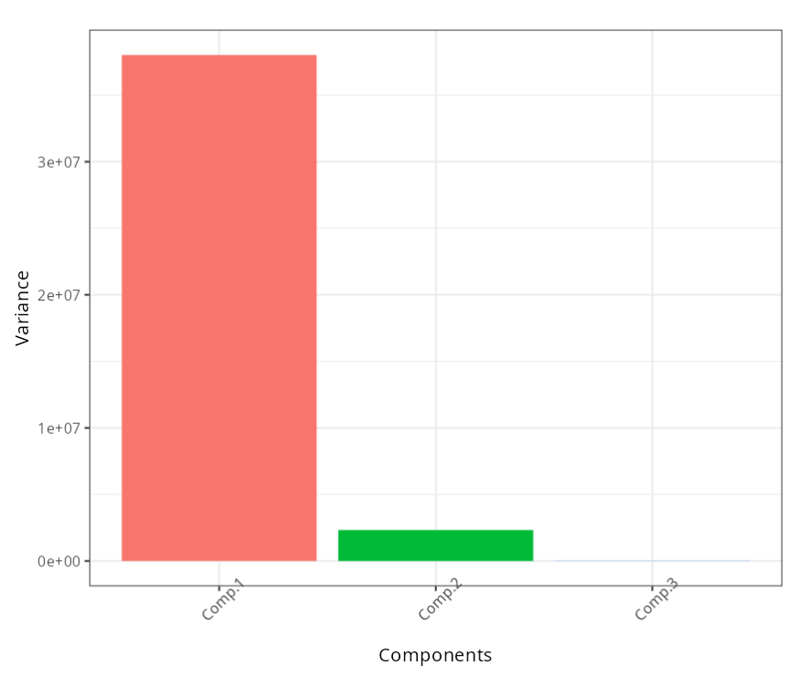
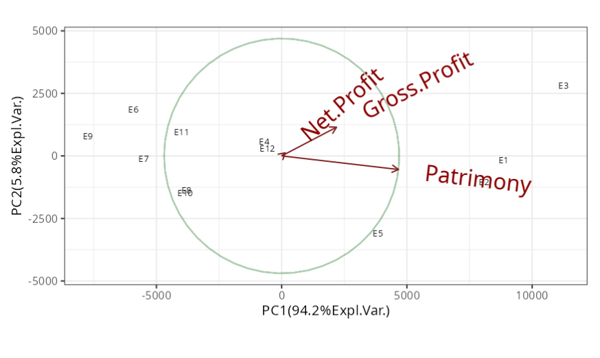
The first principal component explains 94.18% of the total variation. The gross earnings and equity have negatively high weights in the first principal component, -0.425 and -0.905 respectively. the first principal component, -0.425 and -0.905 respectively. variable has practically no effect on this component, as its its weight is very low, -0.02.
Thus, the first component can be interpreted as an index of the companies' overall performance. Since the weights are negative, the higher the company’s gross profit and equity, the lower the value of this component and the better the company’s overall performance index. Companies E3, E1 and E2 had the best performance indexes, respectively, while the company with the worst index was E9.
Example 2:
Five judges evaluated 8 brands of chicken coxinha in terms of taste, aroma, quality of the dough and quality of the filling. Each judge gave a score from 1 to 5 representing the quality of the coxinhas. The table shows the judges' scores for the quality of each coxinha brand.
| Mark | Taste | Aroma | Dough | Filling |
|---|---|---|---|---|
| M1 | 2.75 | 4.03 | 2.8 | 2.62 |
| M2 | 3.9 | 4.12 | 3.4 | 3.52 |
| M3 | 3.12 | 3.97 | 3.62 | 3.05 |
| M4 | 4.58 | 4.86 | 4.34 | 4.82 |
| M5 | 3.97 | 4.34 | 4.28 | 4.98 |
| M6 | 3.01 | 3.98 | 2.9 | 2.82 |
| M7 | 4.19 | 4.65 | 4.52 | 4.77 |
| M8 | 3.82 | 4.12 | 3.62 | 3.71 |
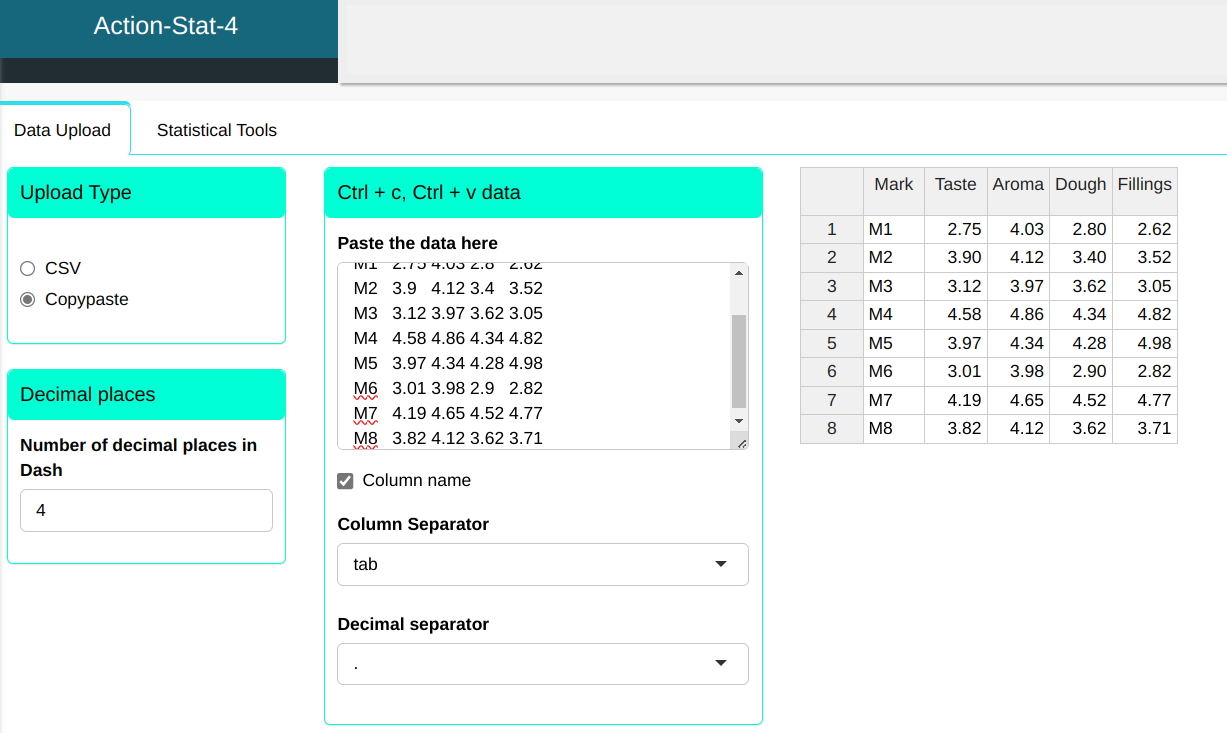
Configuring as shown in the figure below to perform the main component analysis

Then click Calculate to get the results. You can also generate the analyses and download them in Word format.
The results are
Importance of the components
| Information | Comp.1 | Comp.2 | Comp.3 | Comp.4 |
|---|---|---|---|---|
| Standard Deviation | 1.905 | 0.442 | 0.361 | 0.210 |
| Variance Proportion | 0.908 | 0.049 | 0.033 | 0.011 |
| Accumulated Proportion | 0.908 | 0.956 | 0.989 | 1.000 |
Table of component center
| Central Value | |
|---|---|
| Taste | 3.668 |
| Aroma | 4.259 |
| Dough | 3.685 |
| Filling | 3.786 |
Correlation Matrix
| Comp.1 | Comp.2 | Comp.3 | Comp.4 | |
|---|---|---|---|---|
| Comp.1 | 1 | 0 | 0 | 0 |
| Comp.2 | 0 | 1 | 0 | 0 |
| Comp.3 | 0 | 0 | 1 | 0 |
| Comp.4 | 0 | 0 | 0 | 1 |
Analysis Results
| Comp.1 | Comp.2 | Comp.3 | Comp.4 | |
|---|---|---|---|---|
| Taste | 0.499 | 0.153 | 0.825 | 0.216 |
| Aroma | 0.488 | 0.756 | -0.436 | 0.003 |
| Dough | 0.502 | -0.532 | -0.357 | 0.582 |
| Filling | 0.511 | -0.349 | -0.039 | -0.784 |
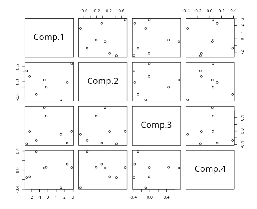
Result of the analysis
| Comp.1 | Comp.2 | Comp.3 | Comp.4 | |
|---|---|---|---|---|
| M1 | -2.523 | 0.437 | -0.378 | -0.154 |
| M2 | -0.410 | 0.075 | 0.695 | 0.045 |
| M3 | -1.386 | -0.498 | -0.281 | 0.384 |
| M4 | 2.838 | 0.721 | -0.011 | 0.053 |
| M5 | 1.554 | -0.711 | -0.097 | -0.371 |
| M6 | -2.187 | 0.216 | -0.016 | -0.141 |
| M7 | 2.302 | -0.028 | -0.359 | 0.126 |
| M8 | -0.187 | -0.212 | 0.447 | 0.059 |
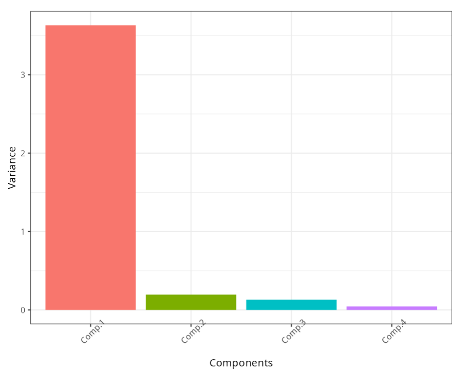
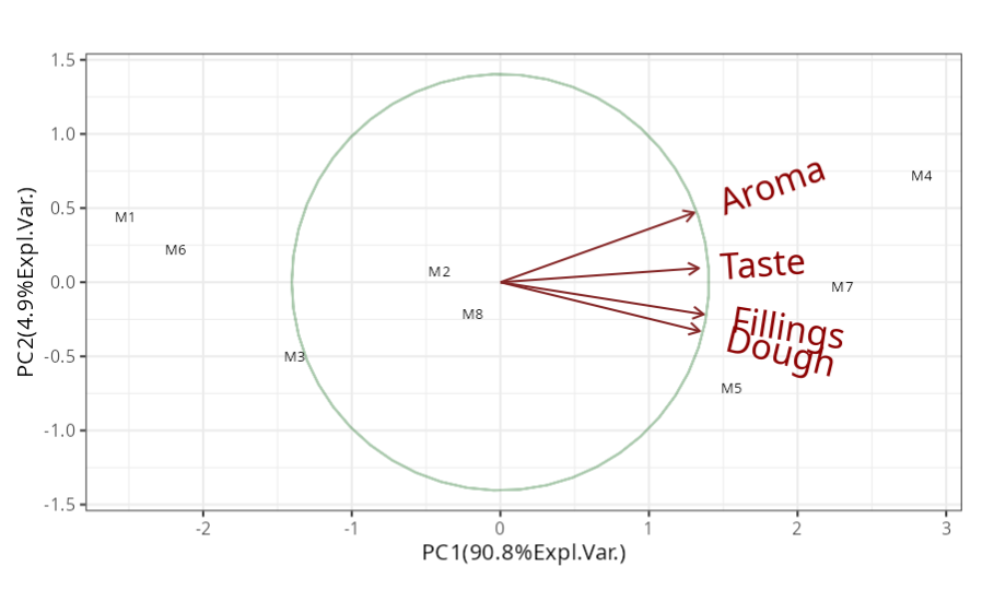
The first principal component explains 90.8% of the total variation and according to the eigenvector table, the weights of the dough, filling, flavor and aroma variables are negatively high for this component, that is, the higher the score of these variables, the lower the score of the first component. Therefore, the first principal component can be understood as a global index of the quality of the coxinha according to the judges.
Thus, a lower score in the first component indicates that the quality index is better, i.e. the lower the score in this component, the better the coxinha. According to the table of scores obtained in this analysis, brands M4, M5 and M7 have the best coxinhas, while brand M1 has the worst coxinha.
Example 3:
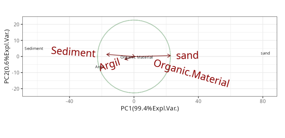
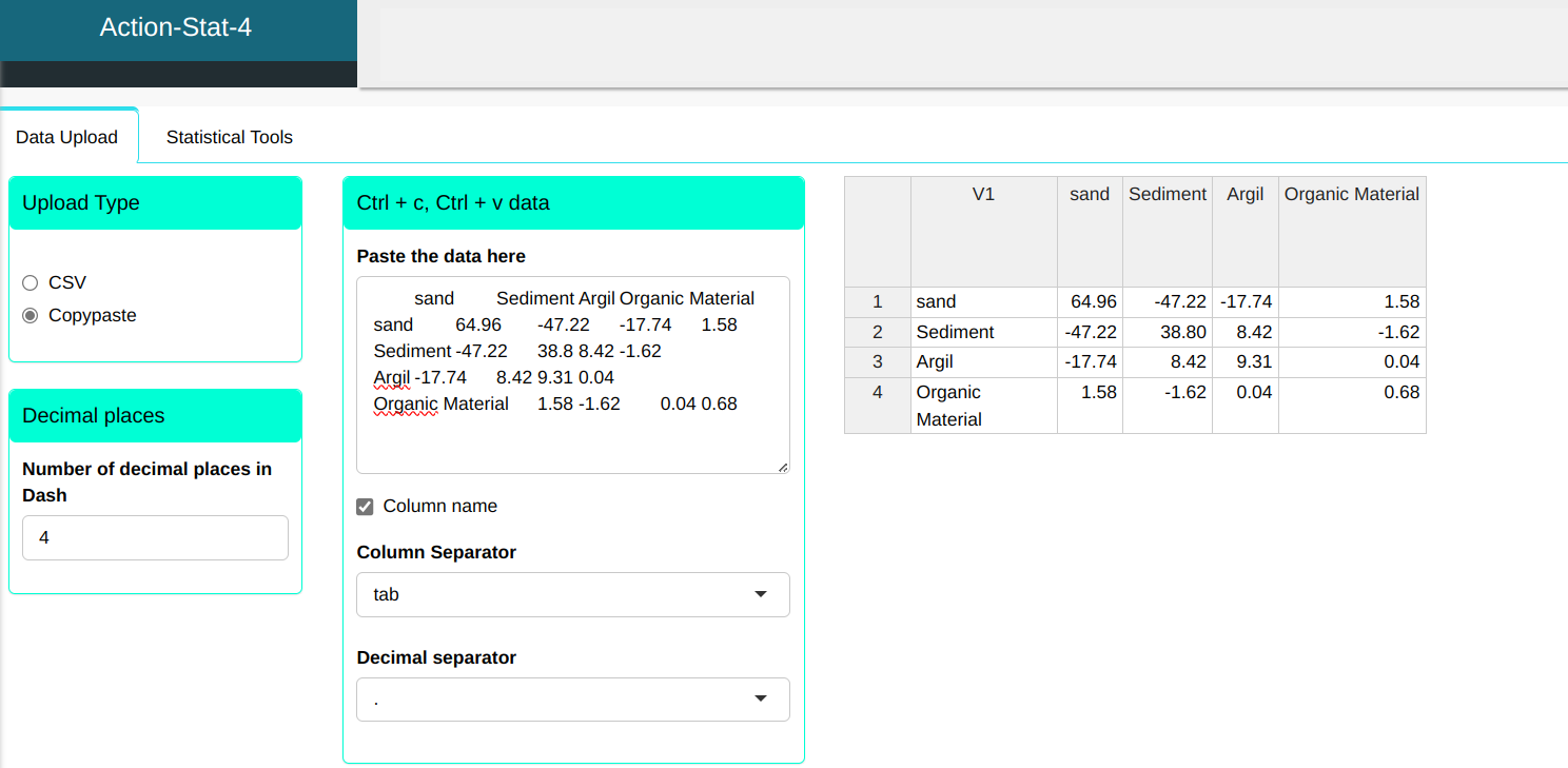
A study collected 25 samples of a particular soil. For each sample, the percentage of sand (X1), sediments (X2), argil (X3) and the amount of organic material (X4) were measured. The covariance matrix of the data analyzed is shown in the table.
| Sand | Sediment | Argil | Organic Material | |
|---|---|---|---|---|
| Sand | 64.96 | -47.22 | -17.74 | 1.58 |
| Sediment | -47.22 | 38.8 | 8.42 | -1.62 |
| Argil | -17.74 | 8.42 | 9.31 | 0.04 |
| Organic Material | 1.58 | -1.62 | 0.04 | 0.68 |
Configuring as shown in the figure below to perform the main component analysis
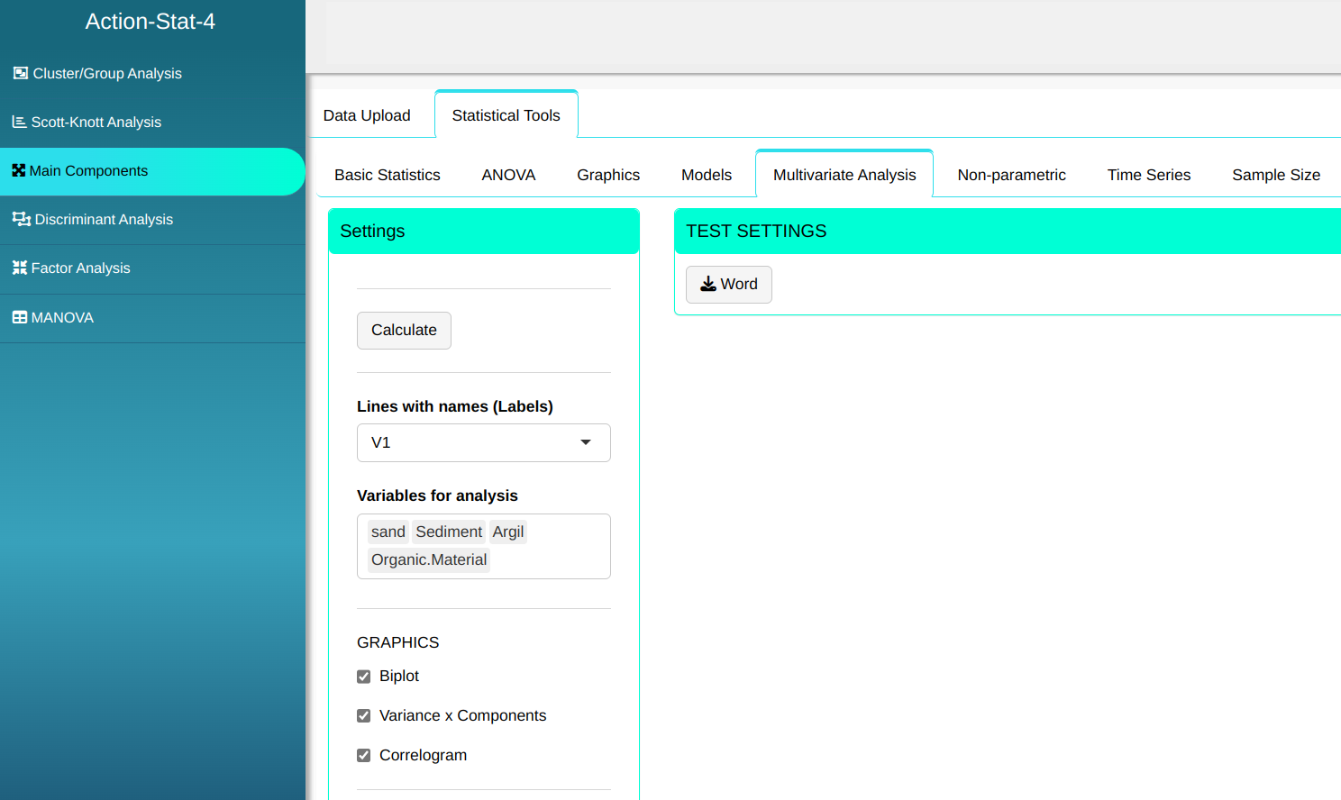

Then click Calculate to get the results. You can also generate the analyses and download them in Word format.
The results are:
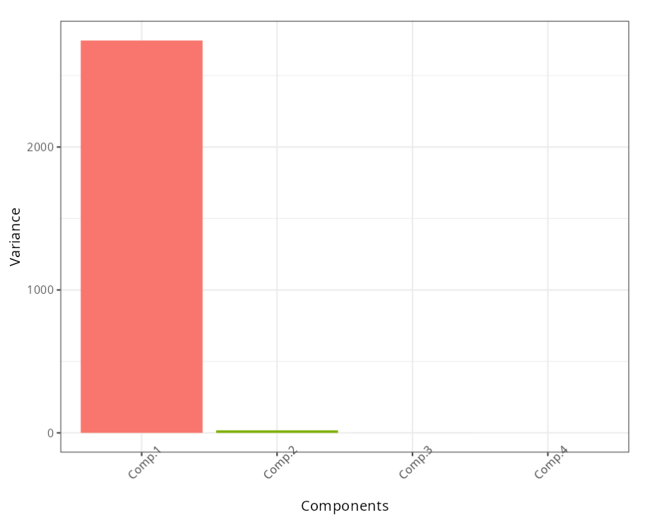
Importance of the components
| Information | Comp.1 | Comp.2 | Comp.3 | Comp.4 |
|---|---|---|---|---|
| Standard Deviation | 52.397 | 4.180 | 0.255 | 0 |
| Variance Proportion | 0.994 | 0.006 | 0.000 | 0 |
| Accumulated Proportion | 0.994 | 1.000 | 1.000 | 1 |
Table of component center
| Central value | |
|---|---|
| Sand | 0.395 |
| Sediment | -0.405 |
| Argil | 0.008 |
| Organic Material | 0.170 |
Correlation Matrix
| Comp.1 | Comp.2 | Comp.3 | Comp.4 | |
|---|---|---|---|---|
| Comp.1 | 1.00 | 0.000 | 0.000 | 0.050 |
| Comp.2 | 0.00 | 1.000 | 0.000 | -0.548 |
| Comp.3 | 0.00 | 0.000 | 1.000 | -0.835 |
| Comp.4 | 0.05 | -0.548 | -0.835 | 1.000 |
Result of the analysis
| Comp.1 | Comp.2 | Comp.3 | Comp.4 | |
|---|---|---|---|---|
| Sand | 0.785 | 0.226 | 0.003 | 0.577 |
| Sediment | -0.587 | 0.565 | 0.057 | 0.577 |
| Argil | -0.198 | -0.790 | -0.053 | 0.578 |
| Organic Material | 0.021 | -0.075 | 0.997 | -0.004 |
Result of the analysis
| Comp.1 | Comp.2 | Comp.3 | Comp.4 | |
|---|---|---|---|---|
| Sand | 81.689 | 2.045 | -0.146 | 0 |
| Sediment | -62.083 | 4.886 | -0.122 | 0 |
| Argil | -21.253 | -6.449 | -0.172 | 0 |
| Organic Material | 1.648 | -0.483 | 0.440 | 0 |