2. Mixed Effect ANOVA
ANOVA is used to analyze the behavior of various treatments of a factor applied to the process and/or product.
Example 1:
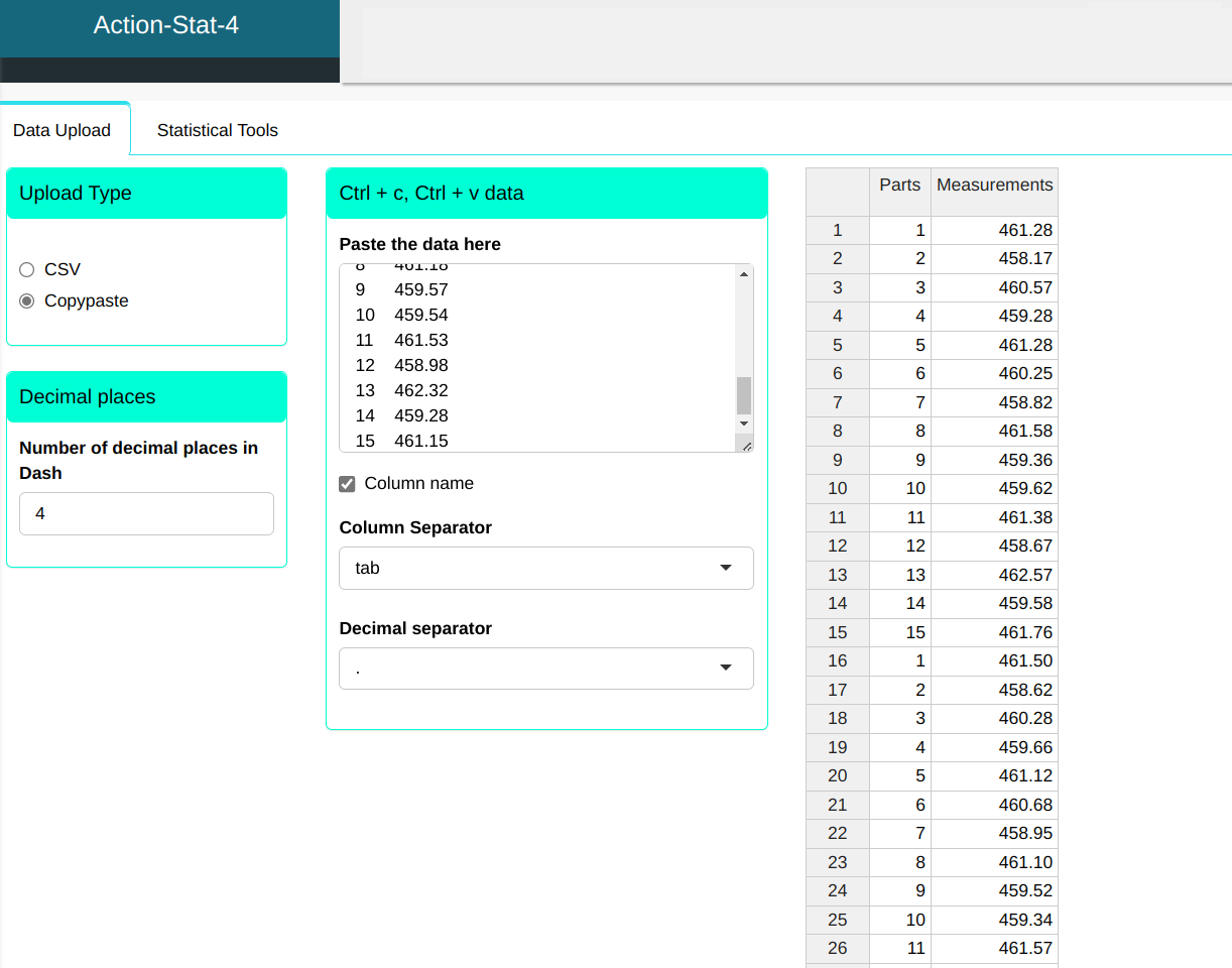
Consider the process of measuring the diameter of a motor bearing. The data are shown below:
| Parts | Measurements |
|---|---|
| 1 | 461.28 |
| 2 | 458.17 |
| 3 | 460.57 |
| 4 | 459.28 |
| 5 | 461.28 |
| 6 | 460.25 |
| 7 | 458.82 |
| 8 | 461.58 |
| 9 | 459.36 |
| 10 | 459.62 |
| 11 | 461.38 |
| 12 | 458.67 |
| 13 | 462.57 |
| 14 | 459.58 |
| 15 | 461.76 |
| 1 | 461.50 |
| 2 | 458.62 |
| 3 | 460.28 |
| 4 | 459.66 |
| 5 | 461.12 |
| 6 | 460.68 |
| 7 | 458.95 |
| 8 | 461.10 |
| 9 | 459.52 |
| 10 | 459.34 |
| 11 | 461.57 |
| 12 | 459.03 |
| 13 | 462.28 |
| 14 | 459.66 |
| 15 | 461.12 |
| 1 | 461.20 |
| 2 | 458.61 |
| 3 | 460.32 |
| 4 | 459.58 |
| 5 | 461.18 |
| 6 | 460.28 |
| 7 | 458.66 |
| 8 | 461.18 |
| 9 | 459.57 |
| 10 | 459.54 |
| 11 | 461.53 |
| 12 | 458.98 |
| 13 | 462.32 |
| 14 | 459.28 |
| 15 | 461.15 |
We will upload the data to the system.
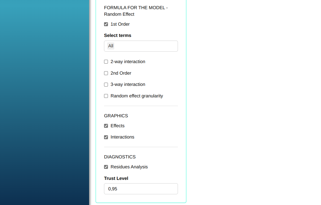
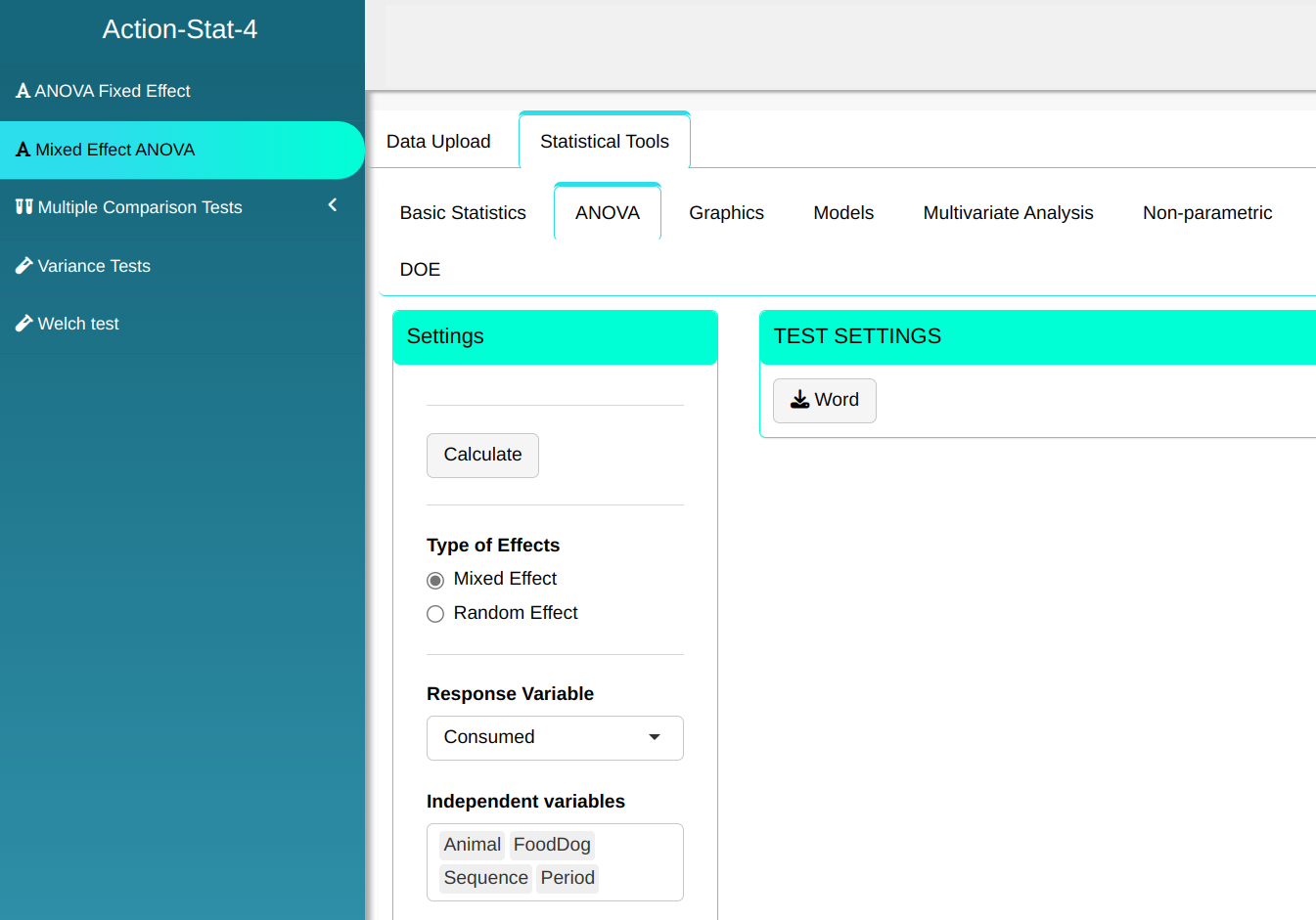
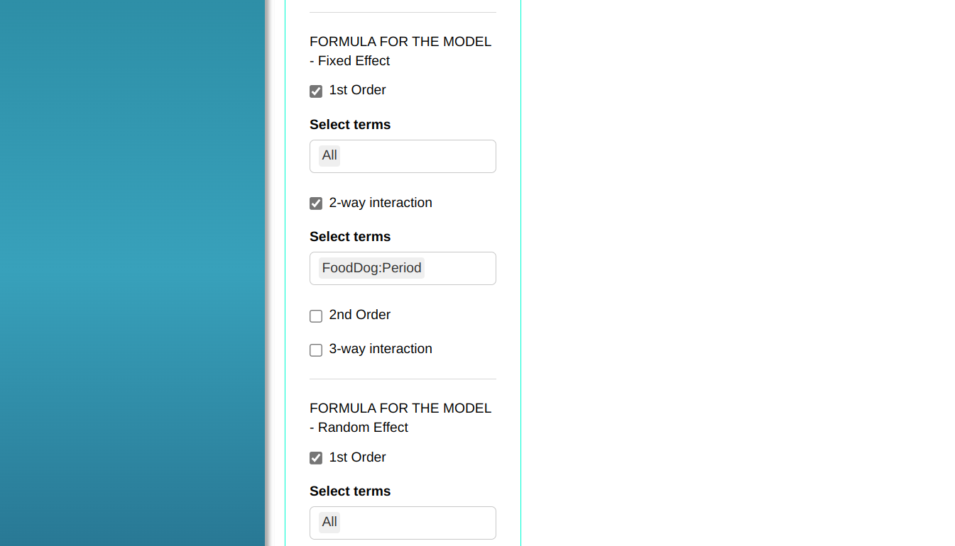
Configuring according to the figure below to perform mixed-effect ANOVA.
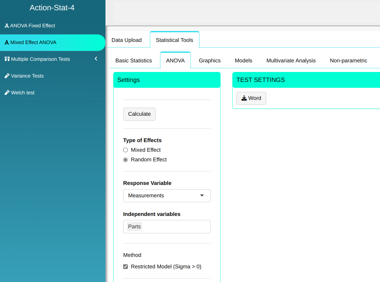
Then click Calculate to get the results. You can also generate the analyses and download them in Word format.

The results are:
Random Effect ANOVA - Restricted Model (Sigma > 0)
| Factors | Standard Deviation | X-squared | DF | P-value | |
|---|---|---|---|---|---|
| X | Pecas | 1.18479 | 91.326 | 1 | 0 |
| X.1 | Resíduos | 0.19707 |
Confidence Interval of the Effect Parts
| Level | Lower Limit | Mean effect | Upper Limit |
|---|---|---|---|
| 1 | 461.094 | 461.327 | 461.559 |
| 2 | 458.234 | 458.467 | 458.699 |
| 3 | 460.158 | 460.390 | 460.622 |
| 4 | 459.274 | 459.507 | 459.739 |
| 5 | 460.961 | 461.193 | 461.426 |
| 6 | 460.171 | 460.403 | 460.636 |
| 7 | 458.578 | 458.810 | 459.042 |
| 8 | 461.054 | 461.287 | 461.519 |
| 9 | 459.251 | 459.483 | 459.716 |
| 10 | 459.268 | 459.500 | 459.732 |
| 11 | 461.261 | 461.493 | 461.726 |
| 12 | 458.661 | 458.893 | 459.126 |
| 13 | 462.158 | 462.390 | 462.622 |
| 14 | 459.274 | 459.507 | 459.739 |
| 15 | 461.111 | 461.343 | 461.576 |
Normality test - Resíduals
| Valor | |
|---|---|
| Mean | 0.000 |
| Standard Deviation | 0.163 |
| N | 45.000 |
| Anderson-Darling | 0.370 |
| P-Value | 0.412 |
Normality Tests - Random Intercept
| Value | |
|---|---|
| Mean | 0.000 |
| Standard Deviation | 1.179 |
| N | 15.000 |
| Anderson-Darling | 0.516 |
| P-Value | 0.159 |
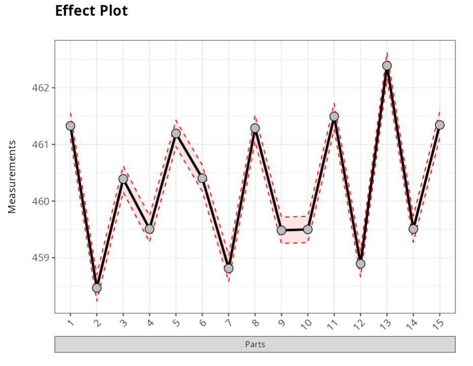
The table released indicates that the parts differ, since the P-value for this factor (Parts) is lower than the predetermined significance level ($\alpha$) of 5%.
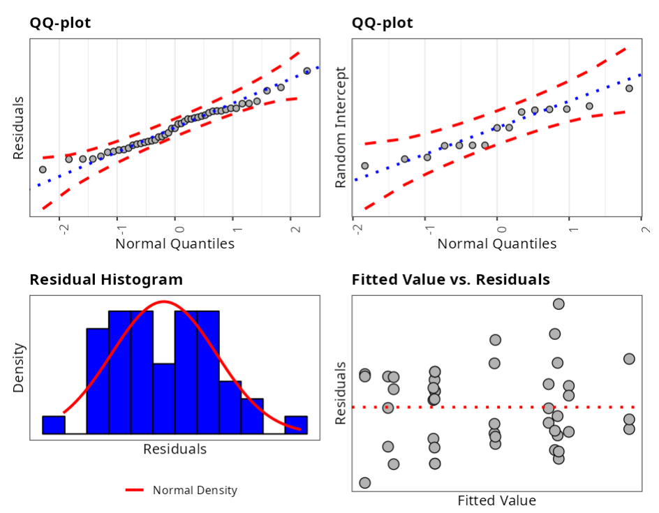
In the graph, the black dots are the mean of each factor level, which in the table are called Effects. The red lines represent the confidence interval for the means of the factor levels.
Graph 1: Graph Residuals versus Normal Quantiles.
Graph 2: Graph the Random Intercept versus Normal Quantiles.
Graph 3: Plots a histogram of the residuals to give us an idea of how the residuals are distributed.
Graph 4: Plots Residuals versus adjusted values.
In our case, we will use the Anderson-Darling test, where the null hypothesis is the normality of the data, and by example, we verify that we do not reject (\“accept\”) the null hypothesis and thus verify the normality of the residuals and the Random Intercept.
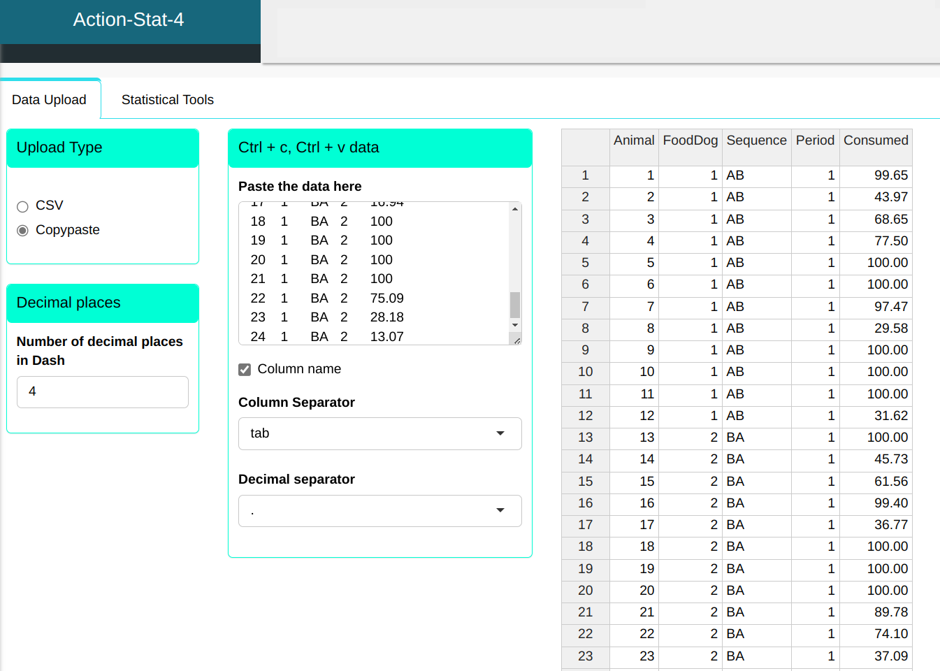
Example 2:
A company wants to test the difference between two types of dog food. 24 animals followed the diet and were evaluated for 6 days. For the first 3 days they were offered one type of food and for the last 3 days another type.
| Animal | Food dog | Sequence | Period | Consumed |
|---|---|---|---|---|
| 1 | 1 | AB | 1 | 99.65 |
| 2 | 1 | AB | 1 | 43.97 |
| 3 | 1 | AB | 1 | 68.65 |
| 4 | 1 | AB | 1 | 77.50 |
| 5 | 1 | AB | 1 | 100.00 |
| 6 | 1 | AB | 1 | 100.00 |
| 7 | 1 | AB | 1 | 97.47 |
| 8 | 1 | AB | 1 | 29.58 |
| 9 | 1 | AB | 1 | 100.00 |
| 10 | 1 | AB | 1 | 100.00 |
| 11 | 1 | AB | 1 | 100.00 |
| 12 | 1 | AB | 1 | 31.62 |
| 13 | 2 | BA | 1 | 100.00 |
| 14 | 2 | BA | 1 | 45.73 |
| 15 | 2 | BA | 1 | 61.56 |
| 16 | 2 | BA | 1 | 99.40 |
| 17 | 2 | BA | 1 | 36.77 |
| 18 | 2 | BA | 1 | 100.00 |
| 19 | 2 | BA | 1 | 100.00 |
| 20 | 2 | BA | 1 | 100.00 |
| 21 | 2 | BA | 1 | 89.78 |
| 22 | 2 | BA | 1 | 74.10 |
| 23 | 2 | BA | 1 | 37.09 |
| 24 | 2 | BA | 1 | 36.08 |
| 1 | 2 | AB | 2 | 100.00 |
| 2 | 2 | AB | 2 | 0.00 |
| 3 | 2 | AB | 2 | 44.97 |
| 4 | 2 | AB | 2 | 43.15 |
| 5 | 2 | AB | 2 | 100.00 |
| 6 | 2 | AB | 2 | 100.00 |
| 7 | 2 | AB | 2 | 100.00 |
| 8 | 2 | AB | 2 | 16.49 |
| 9 | 2 | AB | 2 | 100.00 |
| 10 | 2 | AB | 2 | 100.00 |
| 11 | 2 | AB | 2 | 100.00 |
| 12 | 2 | AB | 2 | 19.10 |
| 13 | 1 | BA | 2 | 0.00 |
| 14 | 1 | BA | 2 | 80.80 |
| 15 | 1 | BA | 2 | 66.98 |
| 16 | 1 | BA | 2 | 100.00 |
| 17 | 1 | BA | 2 | 16.94 |
| 18 | 1 | BA | 2 | 100.00 |
| 19 | 1 | BA | 2 | 100.00 |
| 20 | 1 | BA | 2 | 100.00 |
| 21 | 1 | BA | 2 | 100.00 |
| 22 | 1 | BA | 2 | 75.09 |
| 23 | 1 | BA | 2 | 28.18 |
| 24 | 1 | BA | 2 | 13.07 |
We will upload the data to the system.
Configuring according to the figure below to perform mixed-effect ANOVA.
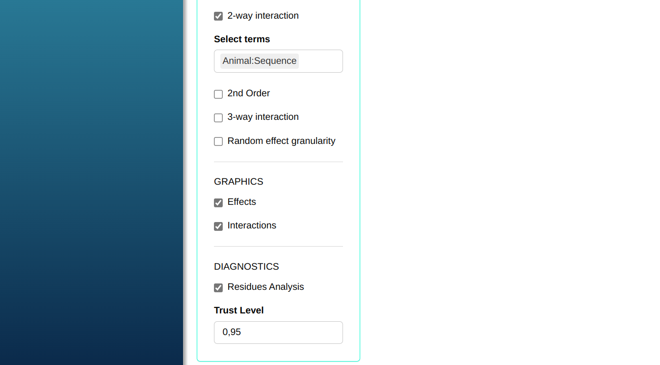
Then click Calculate to get the results. You can also generate the analyses and download them in Word format.
The results are:
Fixed Effect ANOVA
| GL Num. | GL Den. | Sum of Squares | Mean Squares | F Statistics | P-value | |
|---|---|---|---|---|---|---|
| Animal | 1 | 20 | 4.6355 | 4.6355 | 0.0143 | 0.906 |
| FoodDog | 1 | 30.7161 | 11.2679 | 11.2679 | 0.0348 | 0.8533 |
| Sequence | 1 | 20.3385 | 30.252 | 30.252 | 0.0934 | 0.763 |
| Period | 1 | 374.6508 | 253.7175 | 253.7175 | 0.7831 | 0.3768 |
| Animal:Sequence | 1 | 20 | 48.2699 | 48.2699 | 0.149 | 0.7036 |
| FoodDog:Period |
Random Effect ANOVA
| Factor | Fator | Standard Deviation | Correlation | X² | DF | P-value | |
|---|---|---|---|---|---|---|---|
| X | Animal | (Intercept) | 31.1448 | 17.7508 | 1 | 0 | |
| X.1 | FoodDog | (Intercept) | 1.5657 | 0.000 | 1 | 1 | |
| X.2 | Sequence | (Intercept) | 3.6907 | 0.000 | 1 | 1 | |
| X.3 | Period | (Intercept) | 6.4968 | 0.000 | 1 | 1 | |
| X.4 | Residuals | 17.9995 |
Confidence Interval of the Effect Animal
| Level | Lower Limit | Mean eefect | Upper Limit |
|---|---|---|---|
| 1 | 73.430 | 99.825 | 126.220 |
| 2 | -4.410 | 21.985 | 48.380 |
| 3 | 30.415 | 56.810 | 83.205 |
| 4 | 33.930 | 60.325 | 86.720 |
| 5 | 73.605 | 100.000 | 126.395 |
| 6 | 73.605 | 100.000 | 126.395 |
| 7 | 72.340 | 98.735 | 125.130 |
| 8 | -3.360 | 23.035 | 49.430 |
| 9 | 73.605 | 100.000 | 126.395 |
| 10 | 73.605 | 100.000 | 126.395 |
| 11 | 73.605 | 100.000 | 126.395 |
| 12 | -1.035 | 25.360 | 51.755 |
| 13 | 23.605 | 50.000 | 76.395 |
| 14 | 36.870 | 63.265 | 89.660 |
| 15 | 37.875 | 64.270 | 90.665 |
| 16 | 73.305 | 99.700 | 126.095 |
| 17 | 0.460 | 26.855 | 53.250 |
| 18 | 73.605 | 100.000 | 126.395 |
| 19 | 73.605 | 100.000 | 126.395 |
| 20 | 73.605 | 100.000 | 126.395 |
| 21 | 68.495 | 94.890 | 121.285 |
| 22 | 48.200 | 74.595 | 100.990 |
| 23 | 6.240 | 32.635 | 59.030 |
| 24 | -1.820 | 24.575 | 50.970 |
Confidence Interval of the Effect Sequence
| Level | Lower Limit | Mean Effect | Upper Limit |
|---|---|---|---|
| AB | 66.148 | 71.536 | 76.924 |
| BA | 66.148 | 71.536 | 76.924 |
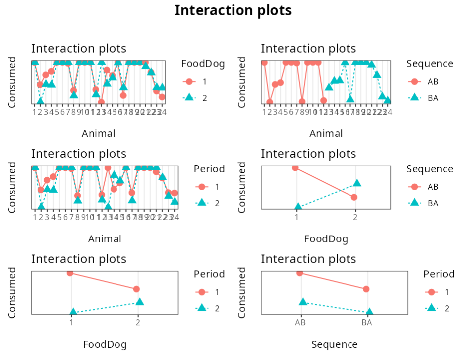
Confidence Interval of the Effect FoodDog*Period
| Level | Lower Limit | Mean Effect | Upper Limit |
|---|---|---|---|
| 1|1 | 67.401 | 76.733 | 86.065 |
| 2|1 | 66.347 | 75.680 | 85.012 |
| 1|2 | 58.060 | 67.392 | 76.724 |
| 2|2 | 57.007 | 66.339 | 75.671 |
Outliers (Quantiles)
| Obs. | Normal Quantiles | Residuals | Criterio |
|---|---|---|---|
| 13 | 2.31 | 42.313 | Envelope (Confidence Level=95%) |
| 37 | -2.31 | -49.400 | Envelope (Confidence Level=95%) |
| 14 | -1.62 | -23.180 | Envelope (Confidence Level=95%) |
| 31 | 1.32 | 9.987 | Envelope (Confidence Level=95%) |
| 4 | 1.45 | 10.234 | Envelope (Confidence Level=95%) |
Normality tests - Residuals
| Value | |
|---|---|
| Mean | 0.000 |
| Standard Deviation | 13.091 |
| N | 48.000 |
| Anderson-Darling | 1.438 |
| P-Value | 0.001 |
Outliers (Quantis)
| Obs | Normal Quantiles | Random Intercept | Criterion |
|---|---|---|---|
| 11 | 0.05 | 20.373 | Envelope (Confidence Level=95%) |
| 20 | 2.04 | 27.658 | Envelope (Confidence Level=95%) |
Normality Tests - Random Intercept
| Value | |
|---|---|
| Mean | 0.000 |
| Standard Deviation | 26.885 |
| N | 24.000 |
| Anderson-Darling | 1.598 |
| P-Value | 0.000 |
If the P-value is less than or equal to the pre-determined significance level, it means that there is a difference between the two types of feed, otherwise there is no difference. In this case, as the p-values are greater than 0.05, we can’t reject the null hypothesis that the feeds are equal, i.e. we can say that the feeds don’t change the amount the animals consume.
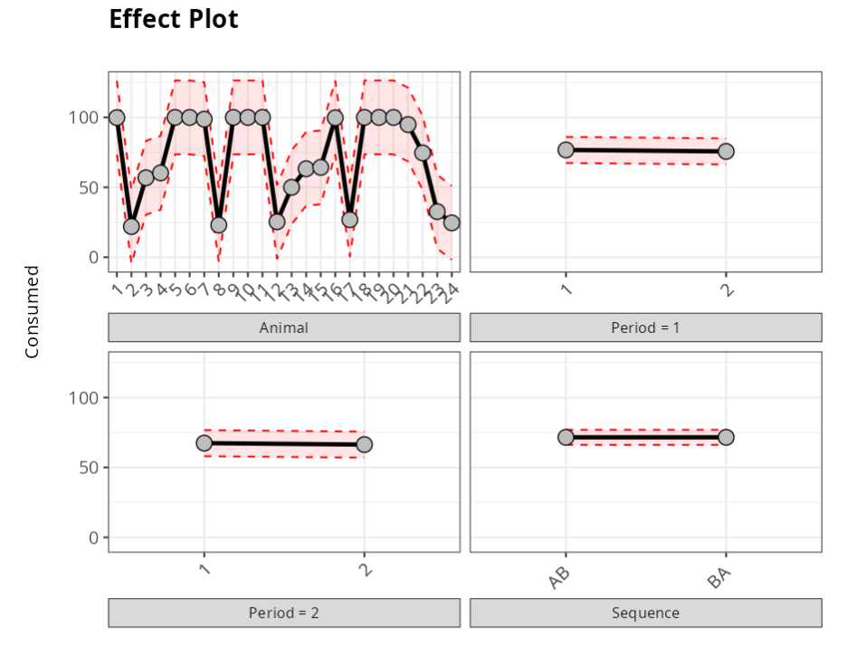
In the graph, the black dots are the means of each factor level, which in the table are called Effects. The red lines represent the confidence interval for the means of the factor levels.
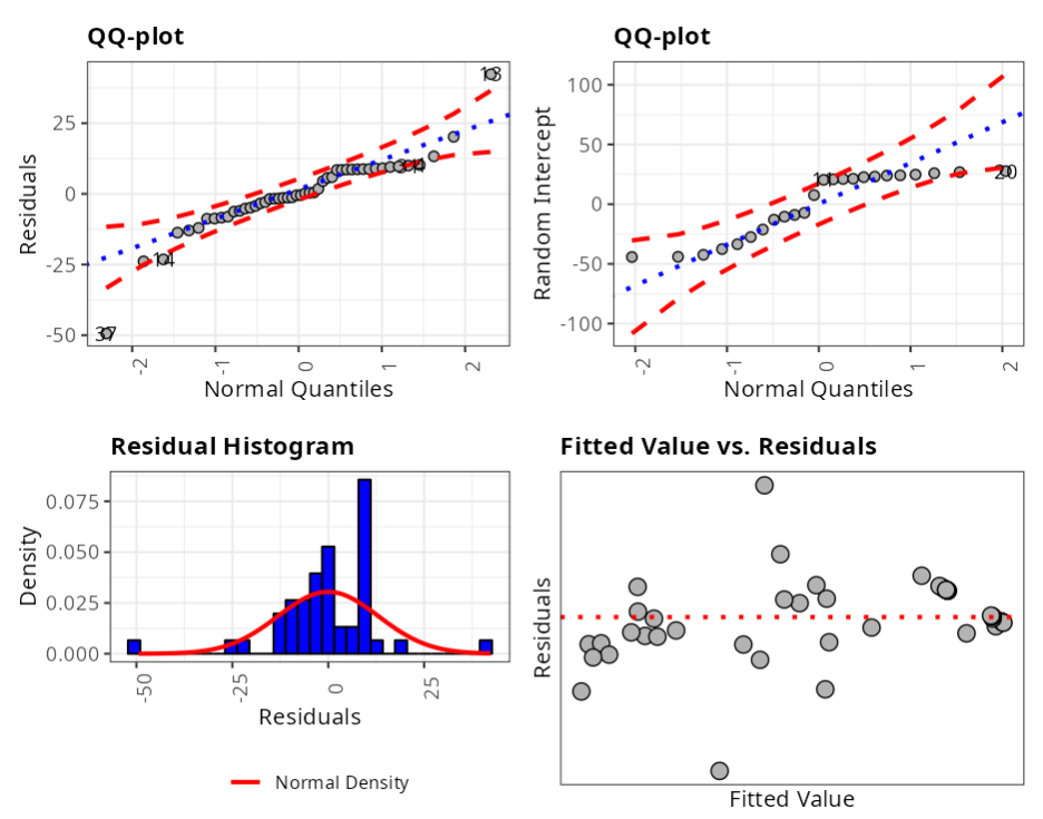
Graph 1: Graph Residuals versus Normal Quantiles.
Graph 2: Graph the Random Intercept versus Normal Quantiles.
Graph 3: Plots a histogram of the residuals to give us an idea of how the residuals are distributed.
Graph 4: Plots Residuals versus adjusted values.
In our case, we will use the Anderson-Darling test, where the null hypothesis is the normality of the data, and by example, we verify that we do not reject (\“accept\”) the null hypothesis and thus verify the normality of the residuals and the Random Intercept.