3. Experiment with Replicas
Through this manual we analyze experiments with replicates and without replicates.
Example 1:
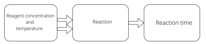
Study the effect on time of a given chemical reaction of varying the temperature and concentration of a reactant, as shown in the diagram below.
| Variable Answer | Y: Reaction time |
|---|---|
| Factors | A: Concentration of Reagent (Levels $V_{-1}$=10% e $V_{+1}$=20%) |
| B: Temperature (levels $T_{-1}$=80ºC e $T_{+1}$=90ºC) | |
| Treatment | $V_{-1}$ $T_{-1}$ - concentration in 10% e temperature in 80ºC ((0)),$\quad$ & |
| $V_{+1}$ $T_{-1}$ - concentration in 20% e temperature in 80ºC (a), | |
| $V_{-1}$ $T_{+1}$ - concentration in 10% e temperature in 90ºC (b) | |
| $V_{+1}$ $T_{+1}$ - concentration in 20% e temperature in 90ºC (ab) | |
| (The number of treatments is 2k, in this case $2^2$=4) | |
| Experimental Unit | Time period for each reaction |
| Replicas | Repetition of the experiment done under the same conditions |
| experimental, in the case of the example under the same temperature | |
| level and reagent. How much more replicas, more reliable the | |
| results of the experiment. |
a) Obtain estimates of the model parameters;
b) Make test of hypothesis to analyze the significance of the parameters.
Build a table as below:
| Treatment | A | B | Y |
|---|---|---|---|
| 0 | -1 | -1 | 26.6 |
| (a) | 1 | -1 | 40.9 |
| (b) | -1 | 1 | 11.8 |
| (ab) | 1 | 1 | 34 |
| 0 | -1 | -1 | 22 |
| (a) | 1 | -1 | 36.4 |
| (b) | -1 | 1 | 15.9 |
| (ab) | 1 | 1 | 29 |
| 0 | -1 | -1 | 22.8 |
| (a) | 1 | -1 | 36.7 |
| (b) | -1 | 1 | 14.3 |
| (ab) | 1 | 1 | 33.6 |
We will upload the data to the system.
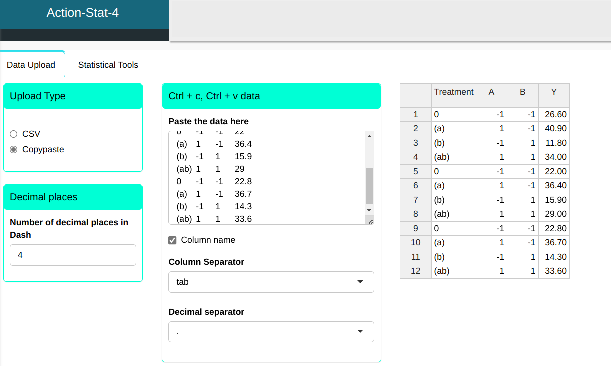
Configure as shown in the figure below to realize the analysis.


Then click Calculate we obtain the results. You can also generate the analyses and download them in Word format.

The results are
ANOVA table
| D.F. | Sum of Squares | Mean Square | F Stat. | P-value | |
|---|---|---|---|---|---|
| A | 1 | 787.32 | 787.320 | 0.894 | 0.367 |
| B | 1 | 182.52 | 182.520 | 0.207 | 0.659 |
| Residuals | 10 | 8808.72 | 880.872 |
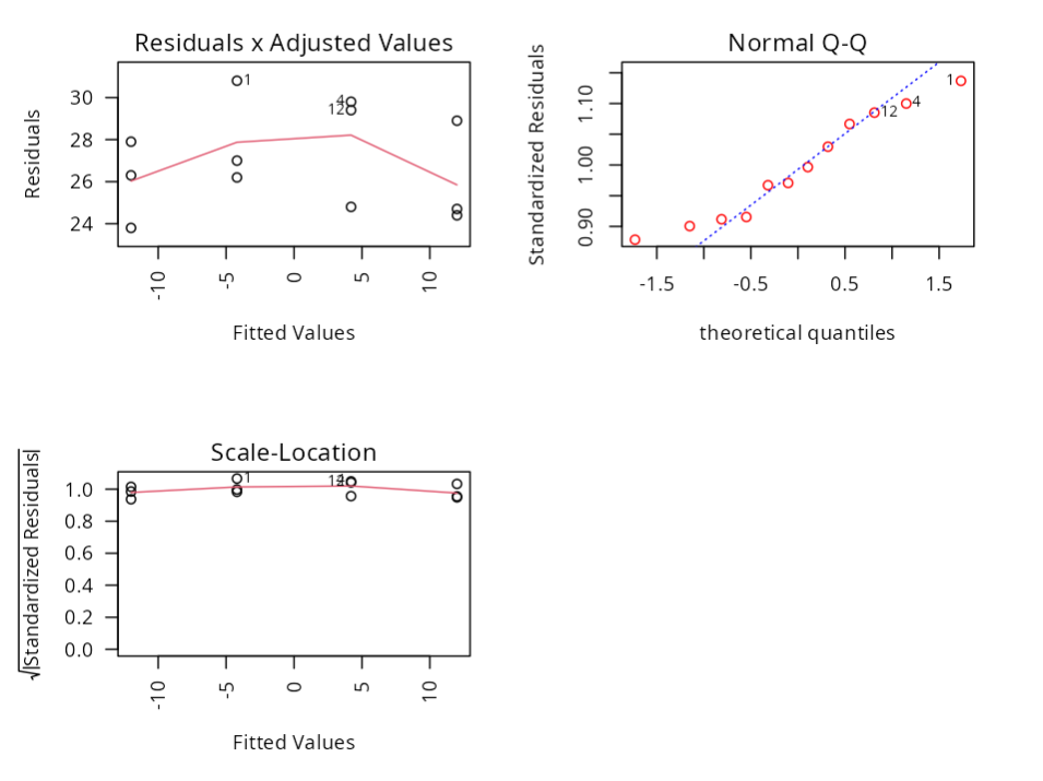
Exploratory Analysis (residues)
| Minimum | 1Q | Median | Mean | 3Q | Maximum |
|---|---|---|---|---|---|
| 23.8 | 24.725 | 26.65 | 27 | 29.275 | 30.8 |
Coefficients
| Effects | Estimate | Standard Deviation | T Stat. | P-value | |
|---|---|---|---|---|---|
| A | 16.2 | 8.1 | 8.568 | 0.945 | 0.367 |
| B | -7.8 | -3.9 | 8.568 | -0.455 | 0.659 |
Descriptive measure for Goodness-of-Fit
| Standard deviation of residuals | Degrees of Freedom | R² | Adjusted R² |
|---|---|---|---|
| 29.679 | 10 | 0.099 | -0.081 |
Confidence interval for the parameters
| 2.5 % | 97.5 % | |
|---|---|---|
| A | -10.99 | 27.19 |
| B | -22.99 | 15.19 |
Prediction Interval
| Y | A | B | Fitted Value | Lower Limit | Upper Limit | Standard Deviation | |
|---|---|---|---|---|---|---|---|
| 1 | 26.6 | -1 | -1 | -4.2 | -31.197 | 22.797 | 12.117 |
| 2 | 40.9 | 1 | -1 | 12 | -14.997 | 38.997 | 12.117 |
| 3 | 11.8 | -1 | 1 | -12 | -38.997 | 14.997 | 12.117 |
| 4 | 34 | 1 | 1 | 4.2 | -22.797 | 31.197 | 12.117 |
| 5 | 22 | -1 | -1 | -4.2 | -31.197 | 22.797 | 12.117 |
| 6 | 36.4 | 1 | -1 | 12 | -14.997 | 38.997 | 12.117 |
| 7 | 15.9 | -1 | 1 | -12 | -38.997 | 14.997 | 12.117 |
| 8 | 29 | 1 | 1 | 4.2 | -22.797 | 31.197 | 12.117 |
| 9 | 22.8 | -1 | -1 | -4.2 | -31.197 | 22.797 | 12.117 |
| 10 | 36.7 | 1 | -1 | 12 | -14.997 | 38.997 | 12.117 |
| 11 | 14.3 | -1 | 1 | -12 | -38.997 | 14.997 | 12.117 |
| 12 | 33.6 | 1 | 1 | 4.2 | -22.797 | 31.197 | 12.117 |
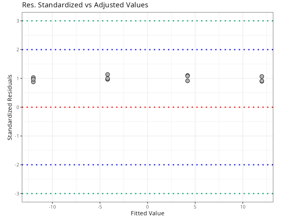
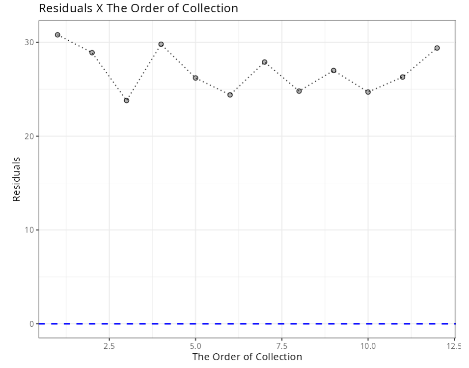
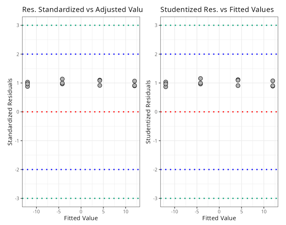
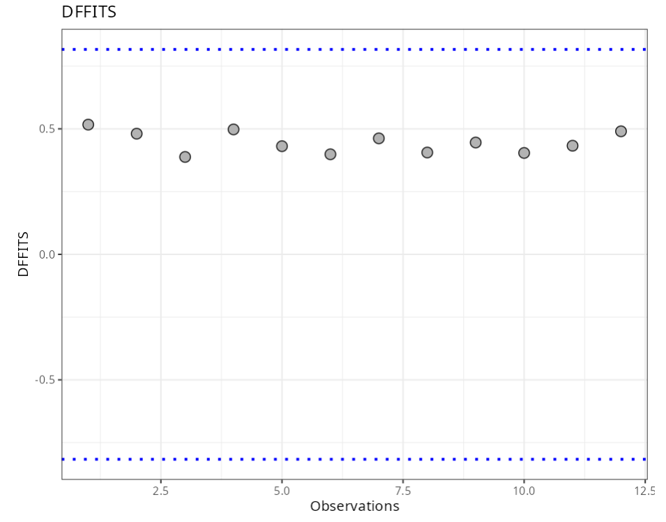
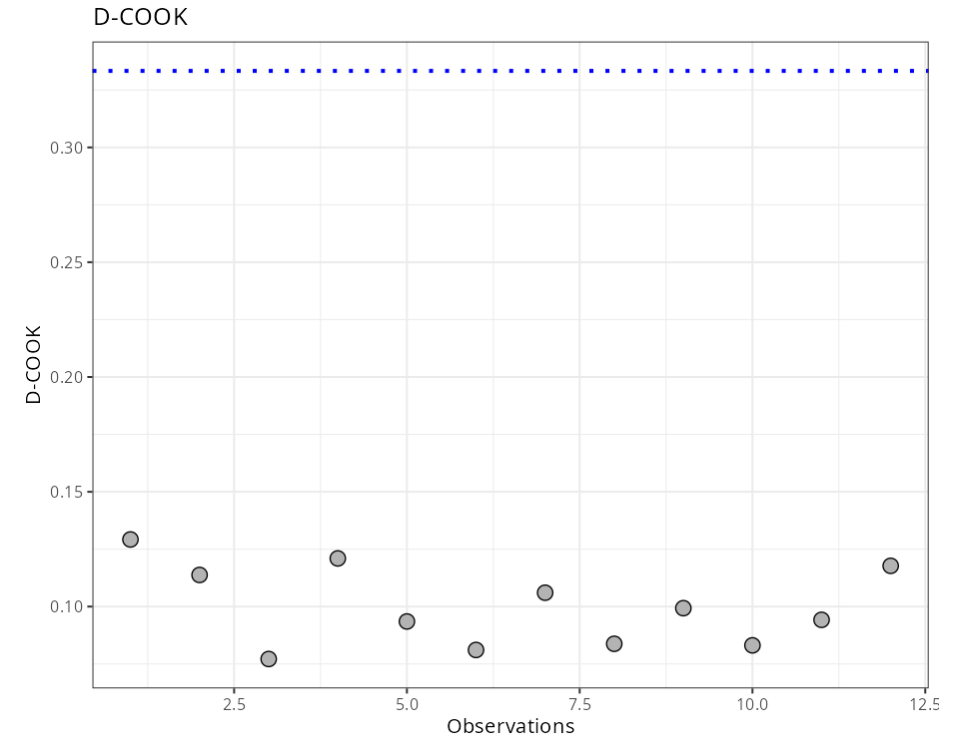
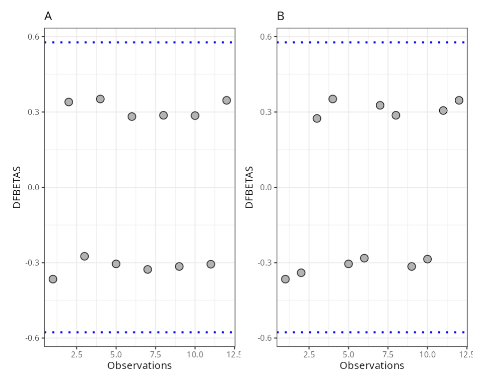
Summary of Residual Analysis
| N.Obs | A | B | Residuals | Studentized Resiaduals | Standardized Residuals | Leverage | DFFITS | DFBETA | D-COOK |
|---|---|---|---|---|---|---|---|---|---|
| 1 | -1 | -1 | 30.8 | 1.156 | 1.137 | 0.167 | 0.517 | -0.365 0.129 | |
| 2 | 1 | -1 | 28.9 | 1.075 | 1.067 | 0.167 | 0.481 | -0.34 | 0.114 |
| 3 | -1 | 1 | 23.8 | 0.868 | 0.878 | 0.167 | 0.388 | 0.274 | 0.077 |
| 4 | 1 | 1 | 29.8 | 1.113 | 1.1 | 0.167 | 0.498 | 0.352 | 0.121 |
| 5 | -1 | -1 | 26.2 | 0.964 | 0.967 | 0.167 | 0.431 | -0.305 0.094 | |
| 6 | 1 | -1 | 24.4 | 0.891 | 0.901 | 0.167 | 0.399 | -0.282 0.081 | |
| 7 | -1 | 1 | 27.9 | 1.033 | 1.03 | 0.167 | 0.462 | 0.327 | 0.106 |
| 8 | 1 | 1 | 24.8 | 0.907 | 0.915 | 0.167 | 0.406 | 0.287 | 0.084 |
| 9 | -1 | -1 | 27 | 0.996 | 0.997 | 0.167 | 0.445 | -0.315 0.099 | |
| 10 | 1 | -1 | 24.7 | 0.903 | 0.912 | 0.167 | 0.404 | -0.286 0.083 | |
| 11 | -1 | 1 | 26.3 | 0.968 | 0.971 | 0.167 | 0.433 | 0.306 | 0.094 |
| 12 | 1 | 1 | 29.4 | 1.096 | 1.085 | 0.167 | 0.49 | 0.347 | 0.118 |
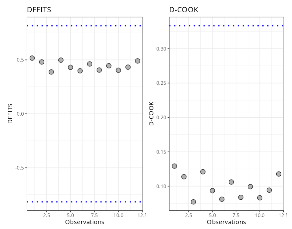
Criterion
| Diagnostic | Formula | Value |
|---|---|---|
| hii (Leverage) | (2*(p+1))/n | 0.330 |
| DFFITS | 2* raíz ((p+1)/n) | 0.820 |
| DCOOK | 4/n | 0.333 |
| DFBETA | 2/raíz(n) | 0.580 |
| Standardized Resiaduals | (-3,3) | 3.000 |
| Studentized Residuals | (-3,3) | 3.000 |
–
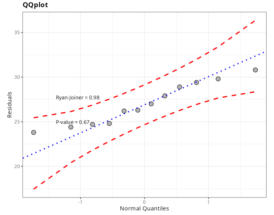
Normality Test
| Statistics | P-value | |
|---|---|---|
| Anderson-Darling | 0.290 | 0.549 |
| Shapiro-Wilk | 0.941 | 0.515 |
| Kolmogorov-Smirnov | 0.159 | 0.552 |
| Ryan-Joiner | 0.979 | 0.669 |
Homoscedasticity Test - Breusch Pagan
| Statistics | DF | P-value |
|---|---|---|
| 0 | 1 | 1 |
Homoscedasticity Test - Goldfeld Quandt
| Variable | Statistics | DF1 | DF2 | P-value |
|---|---|---|---|---|
| A | 0.543762619611975 | 3 | 2 | 0.602191866042602 |
| B | 0.538356274651855 | 3 | 2 | 0.597230105553078 |
Independence Test - Durbin-Watson
| Statistics | P-value |
|---|---|
| 0.0143 | 0 |
Lack of Fit Test
| DF | Sum og square | Mean Square | F Stat. | P-value | |
|---|---|---|---|---|---|
| A | 1 | 787.32 | 787.320 | 129.281 | 0.000 |
| B | 1 | 182.52 | 182.520 | 29.970 | 0.001 |
| Residuals | 10 | 8808.72 | 880.872 | ||
| Lack of Fit | 2 | 8760.00 | 4380.000 | 719.212 | 0.000 |
| Pure Error | 8 | 48.72 | 6.090 |
Analysis Result
| Y | A | B |
|---|---|---|
| 26.6 | -1 | -1 |
| 40.9 | 1 | -1 |
| 11.8 | -1 | 1 |
| 34.0 | 1 | 1 |
| 22.0 | -1 | -1 |
| 36.4 | 1 | -1 |
| 15.9 | -1 | 1 |
| 29.0 | 1 | 1 |
| 22.8 | -1 | -1 |
| 36.7 | 1 | -1 |
| 14.3 | -1 | 1 |
| 33.6 | 1 | 1 |
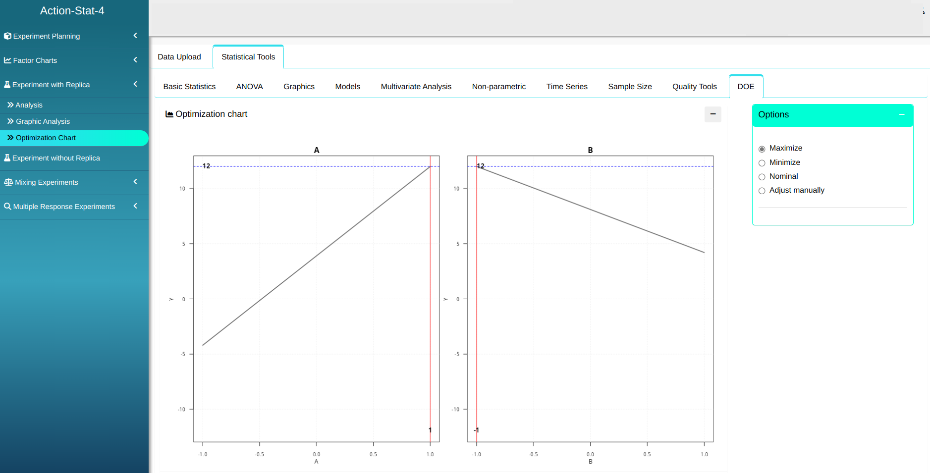
The value of 0.025;12−3−1=2.306 and thus we conclude that, with level α=5%, factors A and B are significant and the interaction AB is not significant. It is enough to see that the regression coefficients of A and B are respectively +1 and -1 and as we are interested in obtaining the smallest response (shortest reaction time), we choose levels A−B+.
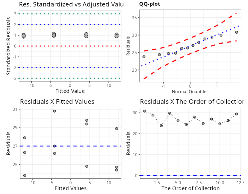
With the results obtained, we can realize a graphical analysis on the system.
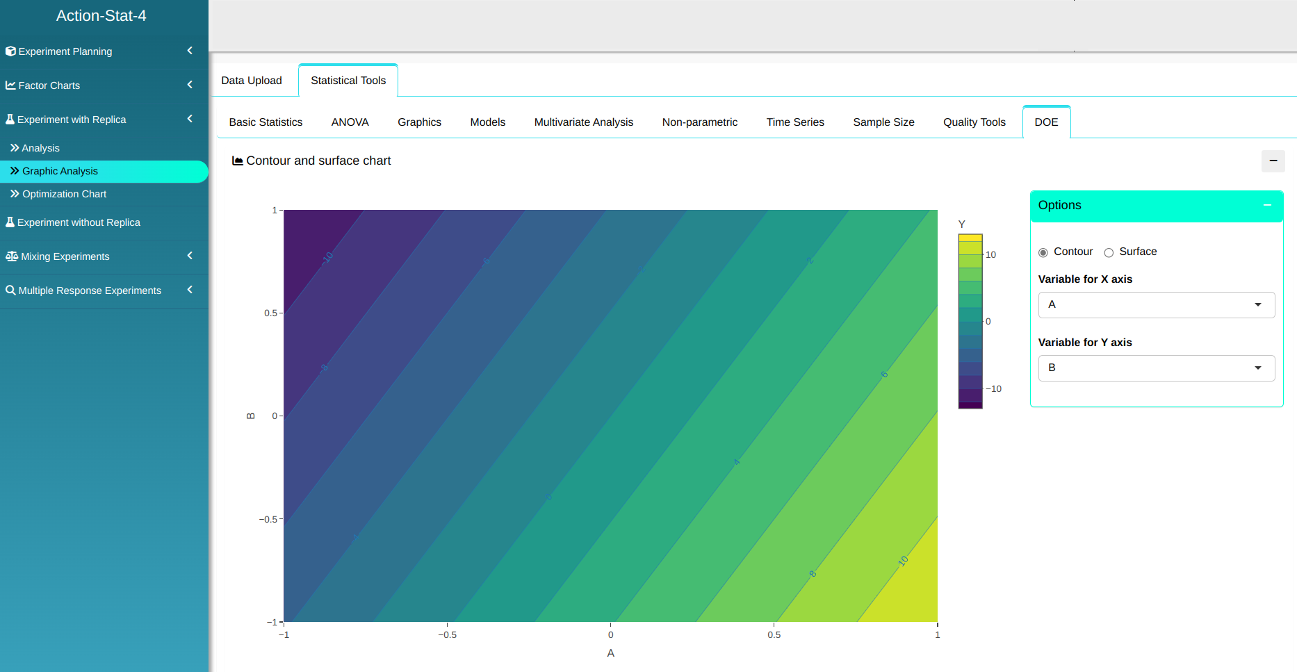
On the same page, you can construct a graph of the feasible region by choosing the upper and lower bound of the answer

Além disso, é possível construir o Gráfico de Otimização.
Example 2:
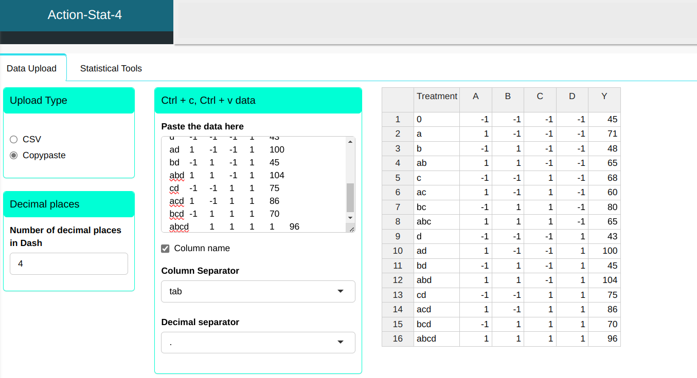
A certain chemical product is produced in a pressure vessel. With the objective of studying study which factors influence the filtration rate of the product (Y), a factorial experiment was carried out in which 4 factors were considered: A (temperature), B (pressure), C (formaldehyde concentration) and D (agitation speed). Each factor is observed at two levels.
| Treatment | A | B | C | D | Y |
|---|---|---|---|---|---|
| 0 | -1 | -1 | -1 | -1 | 45 |
| a | 1 | -1 | -1 | -1 | 71 |
| b | -1 | 1 | -1 | -1 | 48 |
| ab | 1 | 1 | -1 | -1 | 65 |
| c | -1 | -1 | 1 | -1 | 68 |
| ac | 1 | -1 | 1 | -1 | 60 |
| bc | -1 | 1 | 1 | -1 | 80 |
| abc | 1 | 1 | 1 | -1 | 65 |
| d | -1 | -1 | -1 | 1 | 43 |
| ad | 1 | -1 | -1 | 1 | 100 |
| bd | -1 | 1 | -1 | 1 | 45 |
| abd | 1 | 1 | -1 | 1 | 104 |
| cd | -1 | -1 | 1 | 1 | 75 |
| acd | 1 | -1 | 1 | 1 | 86 |
| bcd | -1 | 1 | 1 | 1 | 70 |
| abcd | 1 | 1 | 1 | 1 | 96 |
We will upload the data to the system.
Configure as shown in the figure below to realize the analysis.
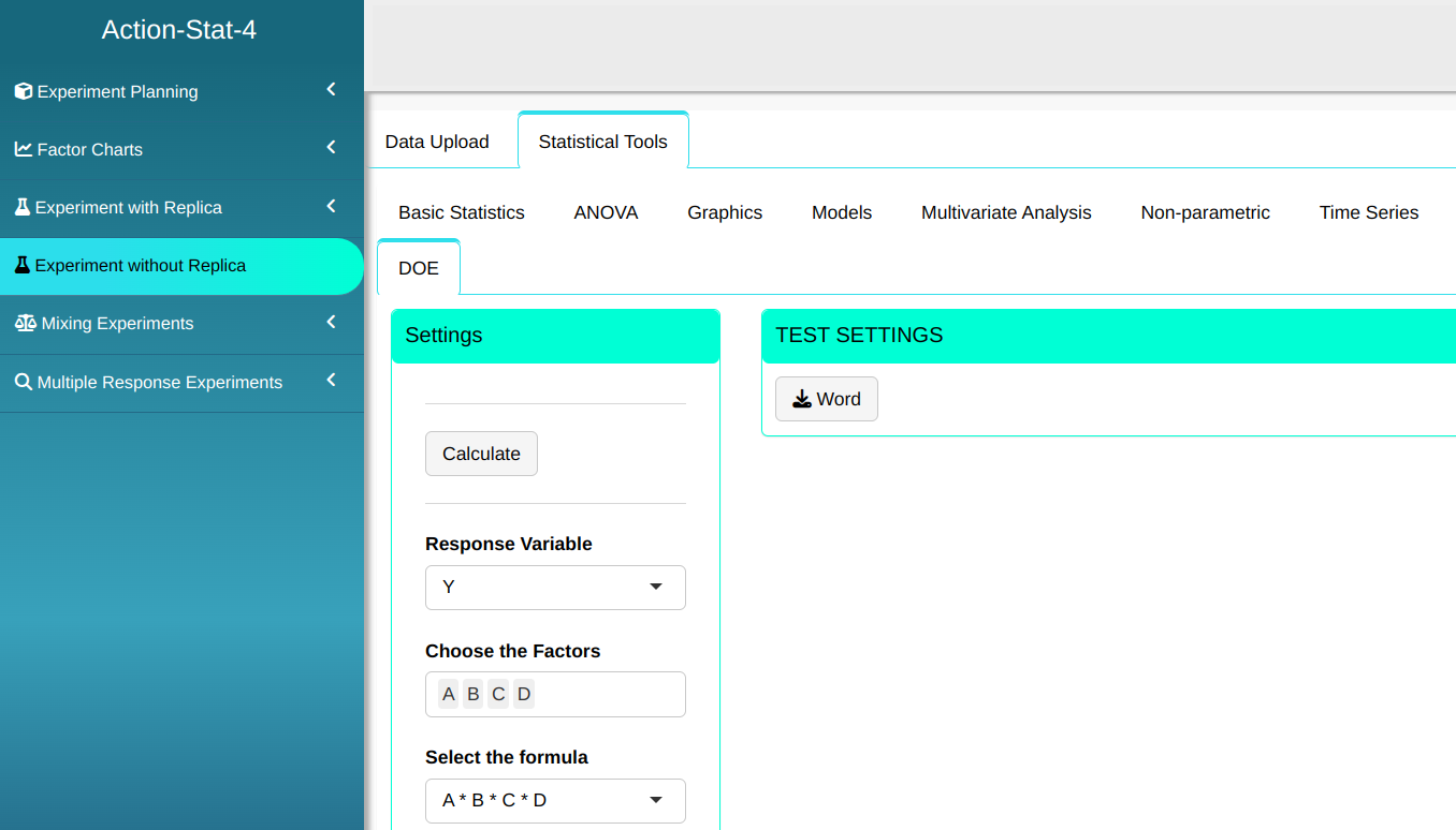

Then click Calculate we obtain the results. You can also generate the analyses and download them in Word format.
The results are
Experiment Analysis without Replication
| Effects | Estimate | Lower Limit | Upper Limit | t Statistic | P-value | |
|---|---|---|---|---|---|---|
| Intercepto | 70.0625 | |||||
| A | 21.6250 | 10.8125 | 14.8772 | 28.3728 | 8.2381 | 0.0004 |
| B | 3.1250 | 1.5625 | -3.6228 | 9.8728 | 1.1905 | 0.2873 |
| C | 9.8750 | 4.9375 | 3.1272 | 16.6228 | 3.7619 | 0.0131 |
| D | 14.6250 | 7.3125 | 7.8772 | 21.3728 | 5.5714 | 0.0026 |
| A:B | 0.1250 | 0.0625 | -6.6228 | 6.8728 | 0.0476 | 0.9639 |
| A:C | -18.1250 | -9.0625 | -24.8728 | -11.3772 | 6.9048 | 0.0010 |
| B:C | 2.3750 | 1.1875 | -4.3728 | 9.1228 | 0.9048 | 0.4071 |
| A:D | 16.6250 | 8.3125 | 9.8772 | 23.3728 | 6.3333 | 0.0014 |
| B:D | -0.3750 | -0.1875 | -7.1228 | 6.3728 | 0.1429 | 0.8920 |
| C:D | -1.1250 | -0.5625 | -7.8728 | 5.6228 | 0.4286 | 0.6861 |
| A:B:C | 1.8750 | 0.9375 | -4.8728 | 8.6228 | 0.7143 | 0.5070 |
| A:B:D | 4.1250 | 2.0625 | -2.6228 | 10.8728 | 1.5714 | 0.1769 |
| A:C:D | -1.6250 | -0.8125 | -8.3728 | 5.1228 | 0.6190 | 0.5630 |
| B:C:D | -2.6250 | -1.3125 | -9.3728 | 4.1228 | 1.0000 | 0.3632 |
| A:B:C:D | 1.3750 | 0.6875 | -5.3728 | 8.1228 | 0.5238 | 0.6228 |
Experiment Analysis withou Replication
| alpha | PSE | ME | SME | t.crit |
|---|---|---|---|---|
| 0.0500 | 2.6250 | 6.7478 | 13.6990 | 2.5706 |
Experiment Analysis withou Replication
| Module Effects | Half-normal score | |
|---|---|---|
| A | 21.6250 | 2.1280 |
| B | 3.1250 | 0.7835 |
| C | 9.8750 | 1.0364 |
| D | 14.6250 | 1.1918 |
| A:B | 0.1250 | 0.0418 |
| A:C | 18.1250 | 1.6449 |
| B:C | 2.3750 | 0.5730 |
| A:D | 16.6250 | 1.3830 |
| B:D | 0.3750 | 0.1257 |
| C:D | 1.1250 | 0.2104 |
| A:B:C | 1.8750 | 0.4770 |
| A:B:D | 4.1250 | 0.9027 |
| A:C:D | 1.6250 | 0.3853 |
| B:C:D | 2.6250 | 0.6745 |
| A:B:C:D | 1.3750 | 0.2967 |
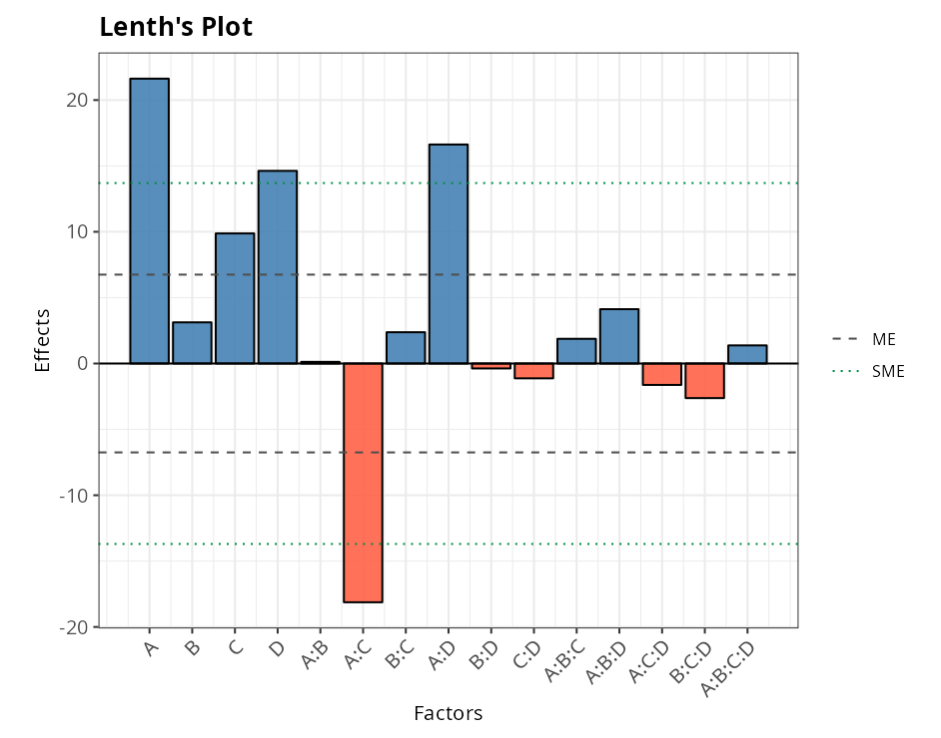
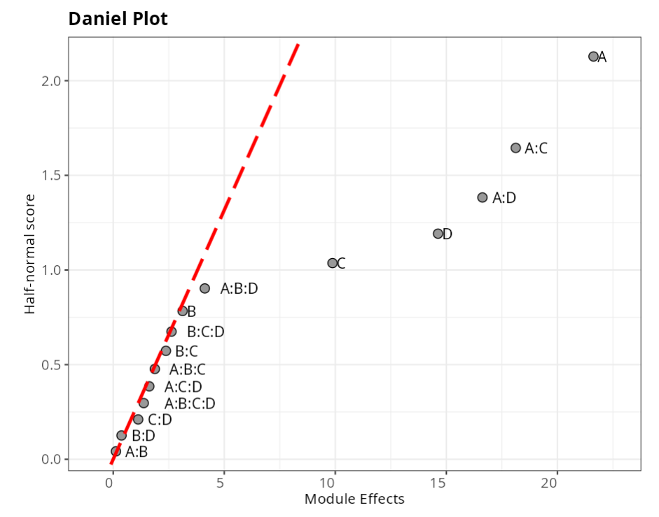
From the results and graphs obtained, we have that factors A, D, and the interactions A:C and A:D are significant.