5. Mixing Experiments

The experiments with Mistura are a special type of experiment in which the factors are ingredients or components of a mixture.

Example:

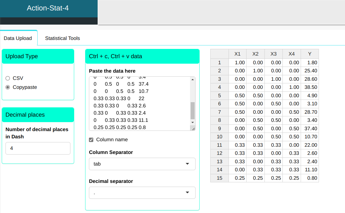
The aim is to reduce the number of mites on a plant. To this end, four types of pesticides, as well as a mixture of them, were sprayed on the plant to analyze the quantity. In the table, xi represents the percentage of pesticide i used in the study, for i=1,2,3,4.

X1	X2	X3	X4	Y
1	0	0	0	1.8
0	1	0	0	25.4
0	0	1	0	28.6
0	0	0	1	38.5
0.5	0.5	0	0	4.9
0.5	0	0.5	0	3.1
0.5	0	0	0.5	28.7
0	0.5	0.5	0	3.4
0	0.5	0	0.5	37.4
0	0	0.5	0.5	10.7
0.33	0.33	0.33	0	22
0.33	0.33	0	0.33	2.6
0.33	0	0.33	0.33	2.4
0	0.33	0.33	0.33	11.1
0.25	0.25	0.25	0.25	0.8

We will upload the data to the system.

Configure as shown in the figure below to realize the analysis.

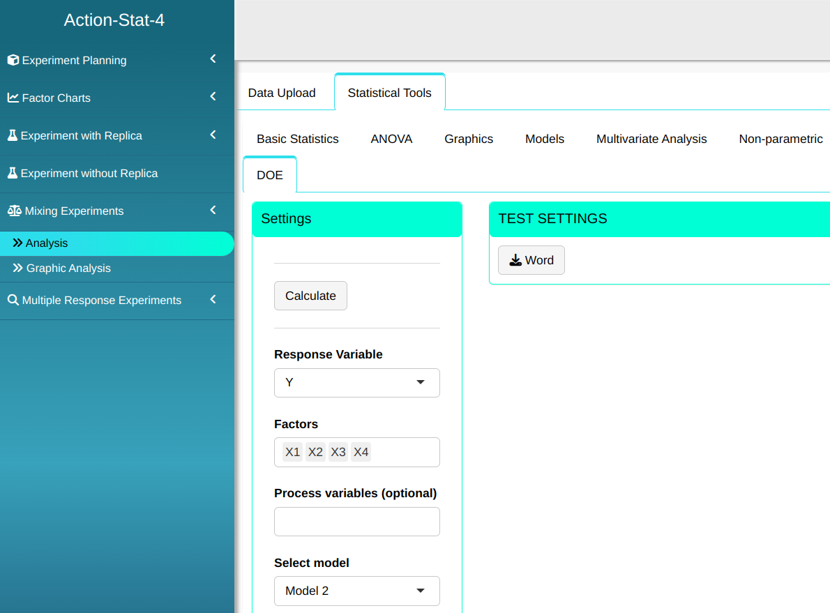
Then click Calculate we obtain the results. You can also generate the analyses and download them in Word format.

The results are

ANOVA table

	D.F.	Sum of Square	Mean Square	F Stat.	P-value
x1	1	400.219	400.219	2.461	0.177
x2	1	1397.90	1397.90	8.596	0.033
x3	1	509.221	509.221	3.131	0.137
x4	1	1883.91	1883.91	11.584	0.019
x1:x2	1	56.413	56.413	0.347	0.581
x1:x3	1	26.98	26.98	0.166	0.701
x1:x4	1	2.001	2.001	0.012	0.916
x2:x3	1	205.057	205.057	1.261	0.312
x2:x4	1	3.108	3.108	0.019	0.895
x3:x4	1	653.163	653.163	4.016	0.101
Residuals	5	813.132	162.626

Coefficients

	Estimate	Standard Deviation	t Stat.	P-value
x1	2.652	12.613	0.21	0.842
x2	25.7	12.613	2.038	0.097
x3	27.947	12.613	2.216	0.078
x4	41.212	12.613	3.267	0.022
x1:x2	-35.951	54.551	-0.659	0.539
x1:x3	-31.917	54.551	-0.585	0.584
x1:x4	-11.573	54.551	-0.212	0.84
x2:x3	-67.701	54.551	-1.241	0.27
x2:x4	-13.758	54.551	-0.252	0.811
x3:x4	-109.324	54.551	-2.004	0.101

Descriptive measure for Goodness-of-Fit

Standard Deviation of residuals	Degrees of Freedom	$\text{R}^2$	Adjusted $\text{R}^2$
12.753	5	0.863	0.59

Summary of Residual analysis

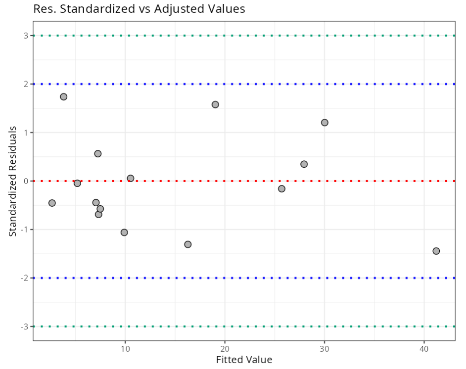
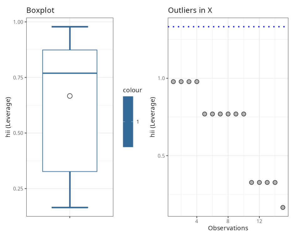
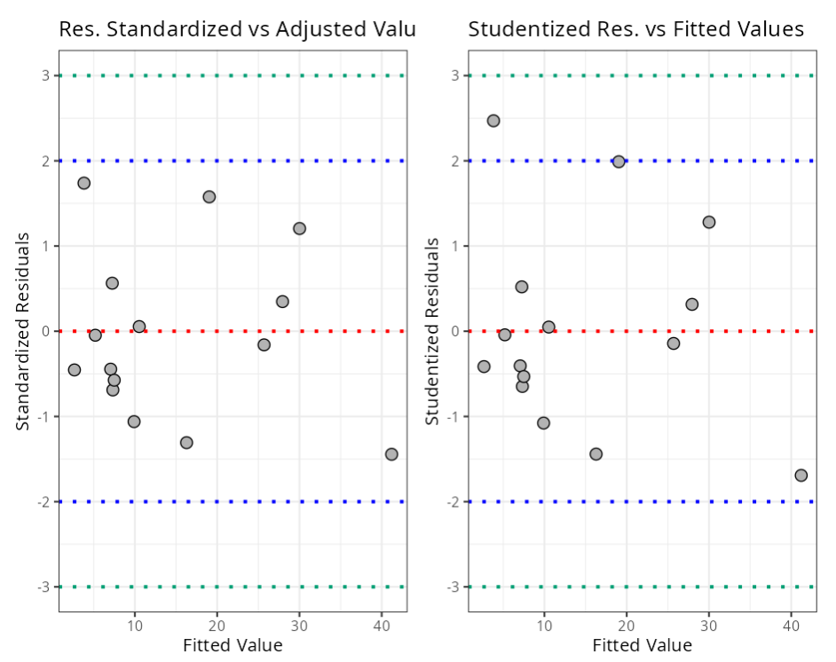
N.Obs	x1	x2	x3	x4	Residuals	Studentized Residuals	Standardized Residuals	Leverage	DFFITS	DFBETA	D-COOK
1	1	0	0	0	-0.852	-0.415	-0.454	0.978	-2.784	0.039	0.929
2	0	1	0	0	-0.3	-0.143	-0.16	0.978	-0.963	-0.963	0.115
3	0	0	1	0	0.653	0.315	0.348	0.978	2.114	-0.03	0.545
4	0	0	0	1	-2.712	-1.692	-1.444	0.978	-11.362	0.159	9.406
5	0.5	0.5	0	0	-0.289	-0.042	-0.047	0.769	-0.077	-0.005	0.001
6	0.5	0	0.5	0	-4.221	-0.648	-0.689	0.769	-1.182	-0.028	0.158
7	0.5	0	0	0.5	9.661	1.989	1.577	0.769	3.631	0.087	0.828
8	0	0.5	0.5	0	-6.498	-1.078	-1.061	0.769	-1.967	-0.122	0.375
9	0	0.5	0	0.5	7.383	1.279	1.205	0.769	2.336	0.145	0.484
10	0	0	0.5	0.5	3.451	0.521	0.563	0.769	0.95	0.023	0.106
11	0.33	0.33	0.33	0	18.185	2.47	1.738	0.327	1.72	-0.135	0.147
12	0.33	0.33	0	0.33	-13.683	-1.442	-1.308	0.327	-1.004	0.079	0.083
13	0.33	0	0.33	0.33	-4.656	-0.406	-0.445	0.327	-0.283	-0.016	0.01
14	0	0.33	0.33	0.33	0.573	0.049	0.055	0.327	0.034	-0.003	0
15	0.25	0.25	0.25	0.25	-6.689	-0.531	-0.574	0.165	-0.236	0.036	0.007

Criterion

Diagnostic	Formula	Value
hii (Leverage)	(2*(p+1))/n	1.300
DFFITS	2* raíz ((p+1)/n)	1.600
DCOOK	4/n	0.267
DFBETA	2/raíz(n)	0.520
Standardized Residuals	(-3,3)	3.000
Student-ized Residuals	(-3,3)	3.000

Normality Test

	Statistic	P-value
Anderson-Darling	0.402	0.315
Shapiro-Wilk	0.949	0.505
Kolmogorov-Smirnov	0.199	0.112
Ryan-Joiner	0.966	0.253

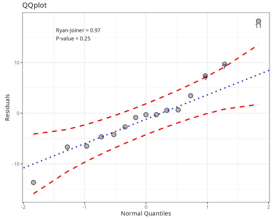
Outliers (Quantiles)

Obs.	Normal Quantiles	Residuals	Criterion
9	0.97	7.38	Envelope (Confidence Level =0.95)
7	1.28	9.66	Envelope (Confidence Level =0.95)
11	1.83	18.18	Envelope (Confidence Level =0.95)

Homoscedasticity Test - Breusch Pagan

Statistic	DF	P-value
0.551	1	0.458

Independence Test - Durbin-Watson

Statistic	P-value
2.57	0.269


	Lack of Fit Test
	Input data do not contain replicas.

Outliers (atypical points)

Observation	T-Value	P-value	P-value Bonferroni
11	2.47	0.069	1

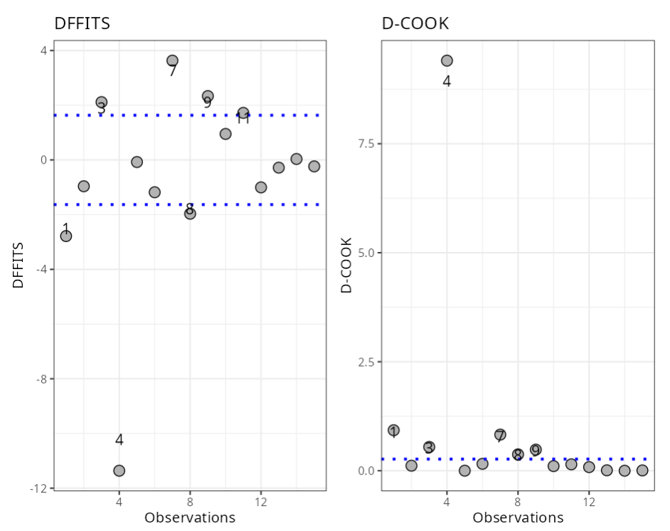
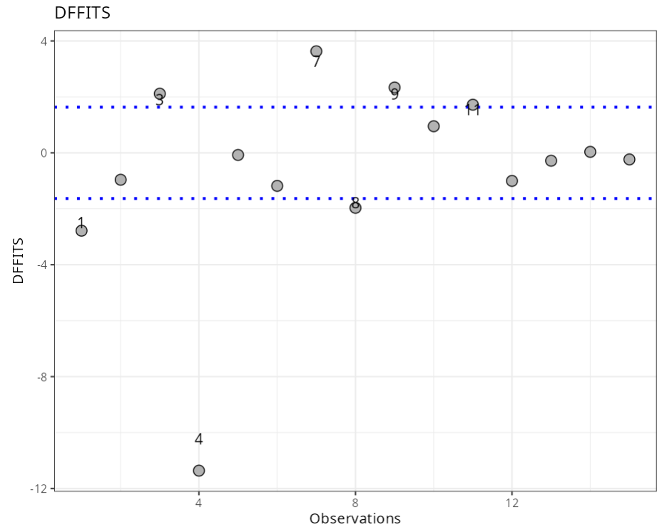
Influential Points

Observations	DFFITS	Criterion
1	-2.78	± 1.63
3	2.11	± 1.63
4	-11.36	± 1.63
7	3.63	± 1.63
8	-1.97	± 1.63
9	2.34	± 1.63
11	1.72	± 1.63

Influential Points

Observations	DCOOK	Criterion
1	0.929	0.267
3	0.545	0.267
4	9.406	0.267
7	0.828	0.267
8	0.375	0.267
9	0.484	0.267

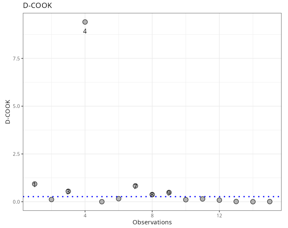
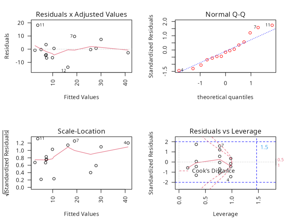
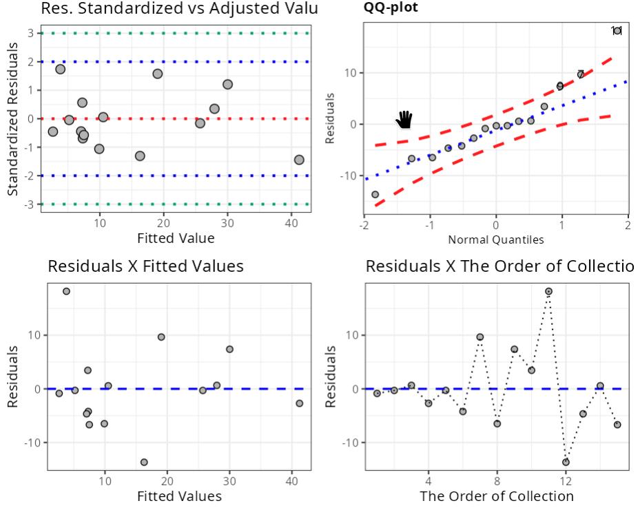
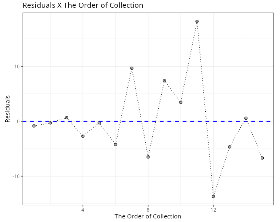
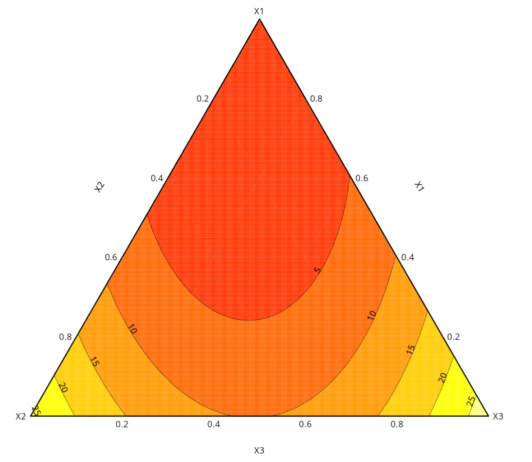
With the calculated results, we can make a graphical analysis.

Clicking on Generate graph the graph will be generated.

Last modified 19.11.2025: Atualizar Manual (288ad71)