6. Multiple Response Experiments

“ACTION” provides this tool that allows you to carry out an Experiment with Multiple Variables and Multiple Responses, and you can create interactive graphs.

Example:

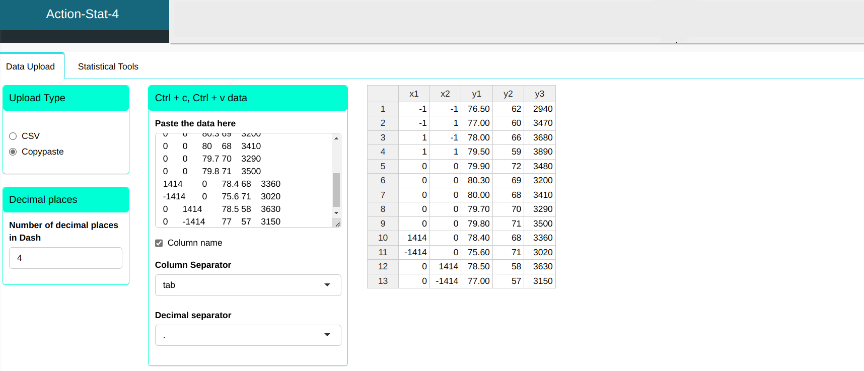
We will carry out the analysis with the following database:

x1	x2	y1	y2	y3
-1	-1	76.5	62	2940
-1	1	77.0	60	3470
1	-1	78.0	66	3680
1	1	79.5	59	3890
0	0	79.9	72	3480
0	0	80.3	69	3200
0	0	80.0	68	3410
0	0	79.7	70	3290
0	0	79.8	71	3500
1414	0	78.4	68	3360
-1414	0	75.6	71	3020
0	1414	78.5	58	3630
0	-1414	77.0	57	3150

---

We will upload the data to the system.

To realize the analysis, simply access DOE and select the options as shown in the figure below.

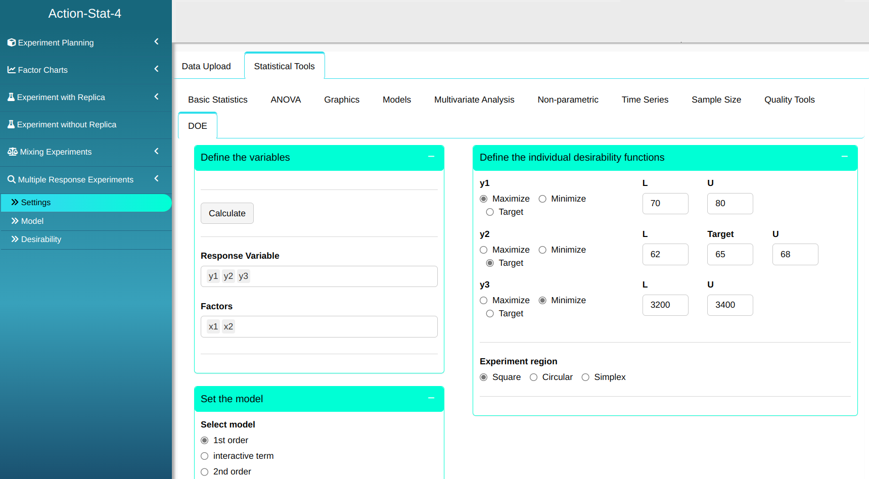
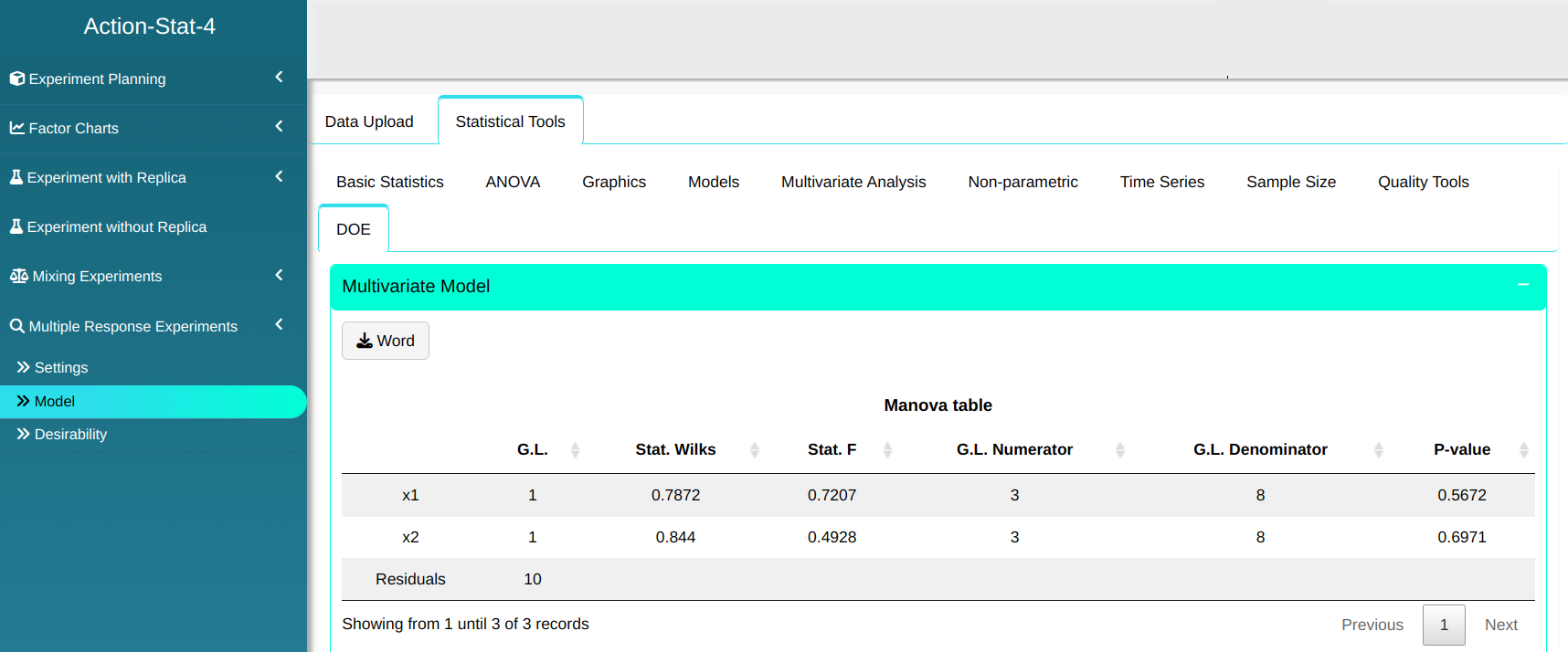
Clicking on Calculate, we can see the results in the “Models” tab And download the results in Word format.

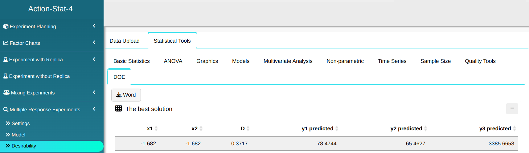
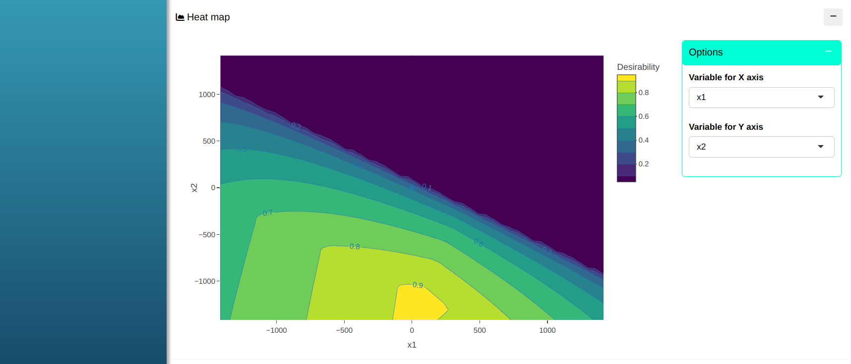
Clicking on the “Desirability” menu shows the best solution along with the heat map.

The results are

Manova Table

	D.F.	Stat. Wilks	Stat. F	D.F. Numerator	D.F. Denominator	P-value
x1	1	0.7872343	0.7207196	3	8	0.5671869
x2	1	0.8440357	0.4927573	3	8	0.6971357
Residuals	10

---

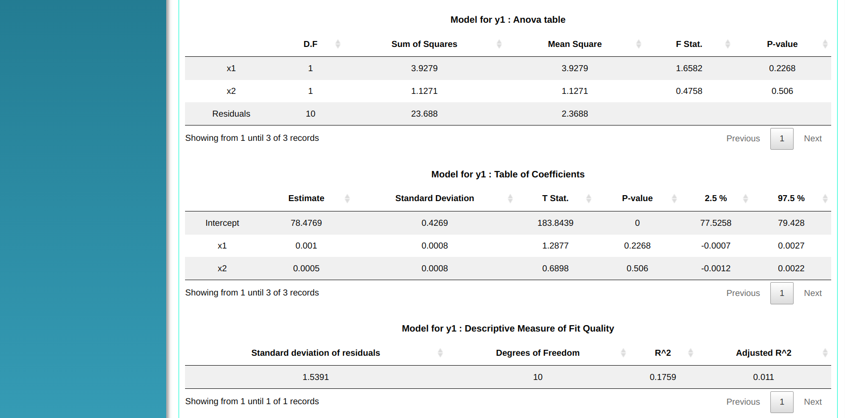
Model for y1: Anova Table

	D.F.	Sum of Squares	Medium Square	Stat. F	P-value
x1	1	3.927921	3.927921	1.6581877	0.2268496
x2	1	1.127122	1.127122	0.4758189	0.5060141
Residuals	10	23.688035	2.368803

---

Model for y1: Table of Coefficient

	Estimate	Deviation.Standard	T. Stat.	P-value	2.5 %	97.5%
Intercept	78.4769	0.4269	183.8439	0	77.5258	79.428
x1	0.001	0.0008	1.2877	0.2268	-0.0007	0.0027
x2	0.0005	0.0008	0.6898	0.506	-0.0012	0.0022

---

Model for y1: Descriptive Measure of Fit Quality

Standard Deviation of residuals	Degrees of Freedom	R²	Adjusted R²
1.539092	10	0.175869	0.01104389

---

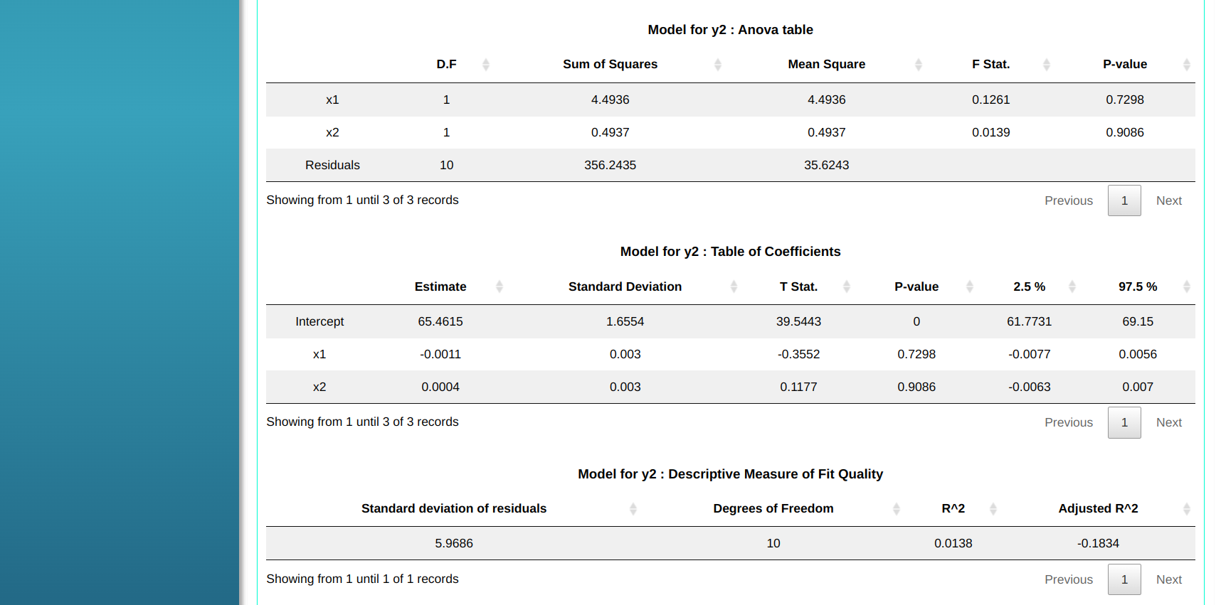
Model for y2: Anova Table

	D.F.	Sum of Squares	Mean Square	F.Stat.	P-value
x1	1	4.4936328	4.4936328	0.12613937	0.7298457
x2	1	0.4936548	0.4936548	0.01385723	0.9086230
Residuals	10	356.2434816	35.6243482

---

Model for y2: Table Coefficient

	Estimate	Deviation.Standard	t. Stat.	P-value	2.5%	97.5%
Intercept	65.4615	1.6554	39.5443	0	61.7731	69.15
x1	-0.0011	0.003	-0.3552	0.7298	-0.0077	0.0056
x2	0.0004	0.003	0.1177	0.90861	-0.0063	0.007

---

Model for y2: Descriptive Measure of Fit Quality

Standard Deviation of residuals	Degrees of Freedom	$R^2$	Adjusted $R^2$
5.968614	10	0.0138063 -0.1834323

---

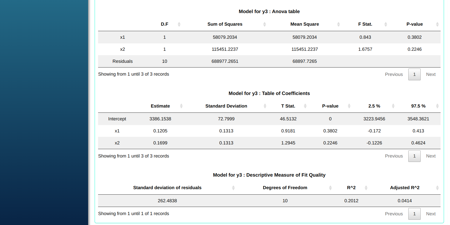
Model for y3: Anova Table

	D.F.	Sum of Squares	Mean Square	F Stat.	P-value
x1	1	58079.2034	58079.2034	0.843	0.3802
x2	1	115451.2237	115451.2237	1.6757	0.2246
Residuals	10	688977.2651	68897.7265

---

Model for y3: Table Coefficient

	Estimate	Standard Deviation	T Stat.	P.value	2.5%	97.5%
Intercept	3386.1538	72.7999	46.5132	0	3223.9456	3548.3621
x1	0.1205	0.1313	0.9181	0.3802	-0.172	0.413
x2	0.1699	0.1313	1.2945	0.2246	-0.1226	0.4624

---

Model for y3: Descriptive Measure of Fit Quality

Standard Deviation of Residuals	Degrees of Freedom	$R^2$	Adjusted $R^2$ Adjusted
262.4838	10	0.201192	0.04143148

---

En la ventana “Deseabilidad” It shows which is the best solution together with the heat map.

---

The best solution

x1	x2	D	y1 Predicted	y2 Predicted	y3 Predicted
-1.682	-1.682	0.3717	78.4744	65.4627	3385.6653

---

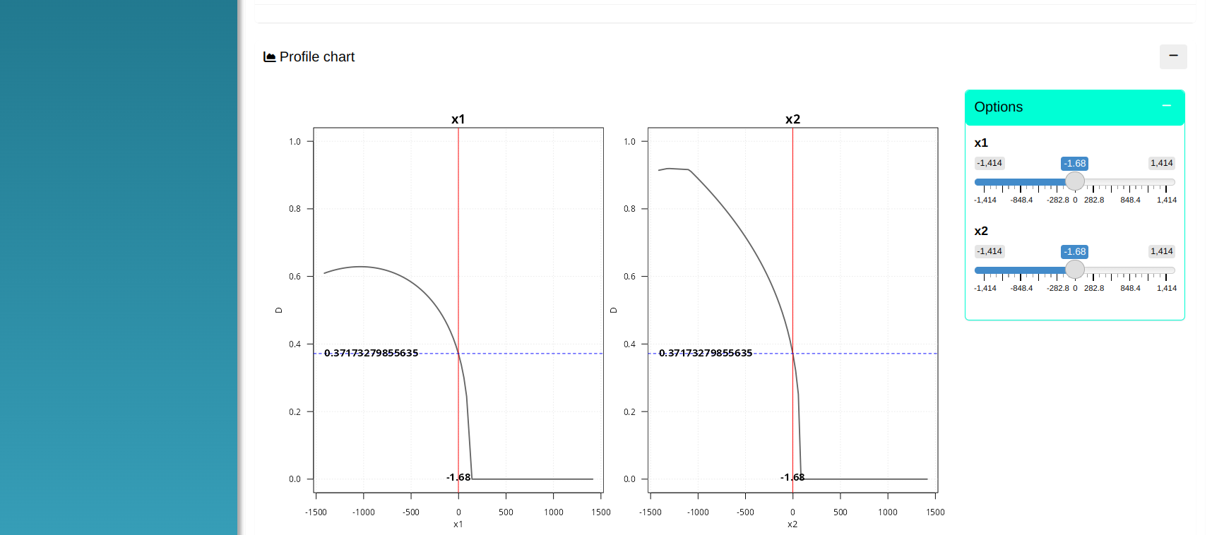
Profile Chart

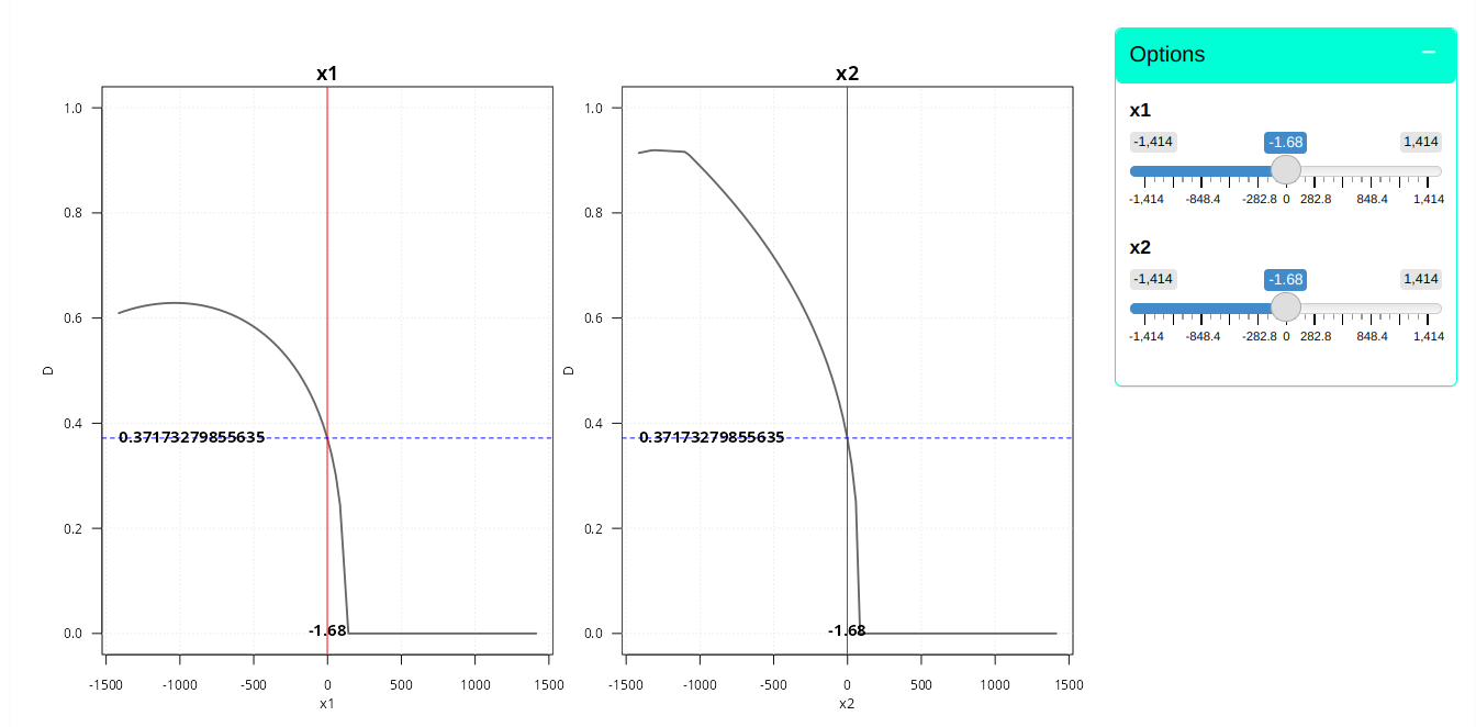
x1	x2	D	y1 Predicted	y2 Predicted	y3 Predicted
-1.68	-1.68	0.37	78.47	65.46	3385.673

---

Heat map

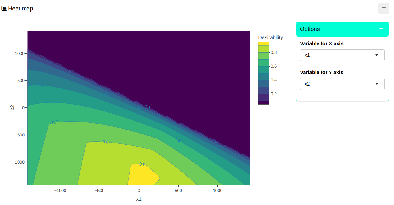
Some solutions

x1	x2	D	y1 Predicted	y2 Predicted	y3 Predicted
0	0	0.3676	78.4769	65.4615	3386.1538

---