15. Distributions
The Action Distributions tool calculates the density, quantile, and percentile of several continuous and discrete distributions.
Example 1:
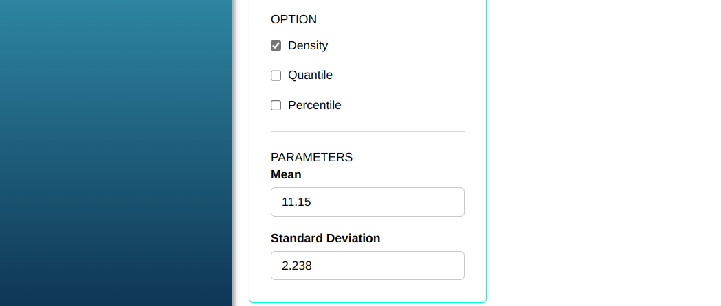
Consider X a Normal random variable with mean 11.15 and deviation standard 2.238. Calculate the probability density.
| 7.57 |
| 12.29 |
| 10.35 |
| 16.28 |
| 11.79 |
| 10.17 |
| 10.77 |
| 11.27 |
| 7.39 |
| 8.25 |
| 8.39 |
| 12.27 |
| 12.82 |
| 12.26 |
| 12.07 |
| 9.72 |
| 8.45 |
| 8.67 |
| 11.17 |
| 8.40 |
| 11.92 |
| 9.39 |
| 9.62 |
| 18.53 |
| 11.67 |
| 8.75 |
| 9.63 |
| 13.06 |
| 4.69 |
| 12.43 |
| 7.69 |
| 10.64 |
| 10.55 |
| 8.85 |
| 6.02 |
| 8.88 |
| 15.46 |
| 12.79 |
| 11.27 |
| 8.01 |
| 9.69 |
| 9.91 |
| 8.43 |
| 12.88 |
| 11.50 |
| 9.82 |
| 14.55 |
| 9.88 |
| 13.25 |
| 10.35 |
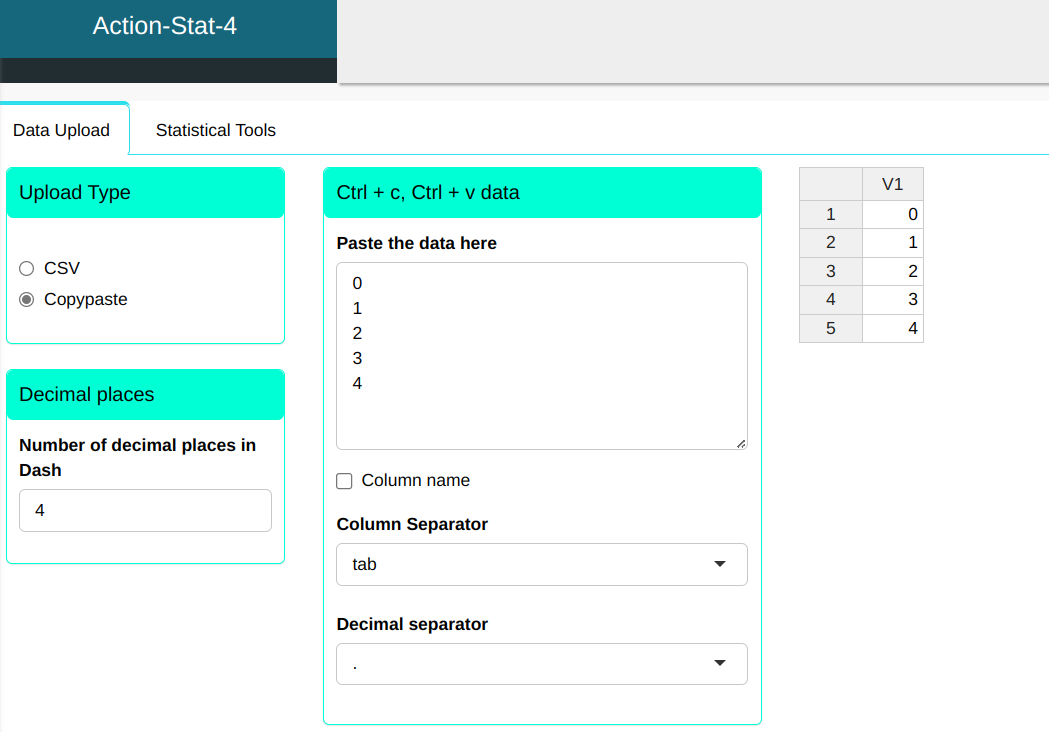
We will upload the data to the system.
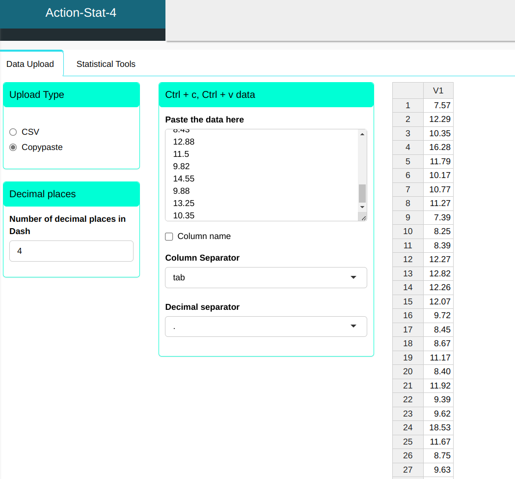
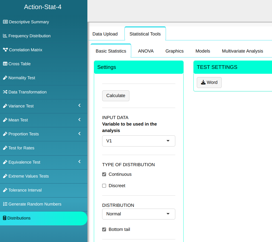
To calculate the probability density, the following setup is performed as shown in the following figure.

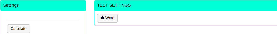
Then click Calculate to get the results. You can also generate the analyses and download them in Word format.
The results are as follows
| Results |
|---|
| 0.050 |
| 0.157 |
| 0.167 |
| 0.013 |
| 0.171 |
| 0.162 |
| 0.176 |
| 0.178 |
| 0.044 |
| 0.077 |
| 0.083 |
| 0.157 |
| 0.135 |
| 0.157 |
| 0.164 |
| 0.145 |
| 0.086 |
| 0.097 |
| 0.178 |
| 0.084 |
| 0.168 |
| 0.131 |
| 0.141 |
| 0.001 |
| 0.174 |
| 0.100 |
| 0.141 |
| 0.124 |
| 0.003 |
| 0.151 |
| 0.054 |
| 0.174 |
| 0.172 |
| 0.105 |
| 0.013 |
| 0.106 |
| 0.028 |
| 0.136 |
| 0.178 |
| 0.066 |
| 0.144 |
| 0.153 |
| 0.085 |
| 0.132 |
| 0.176 |
| 0.150 |
| 0.056 |
| 0.152 |
| 0.115 |
| 0.167 |
Example 2:
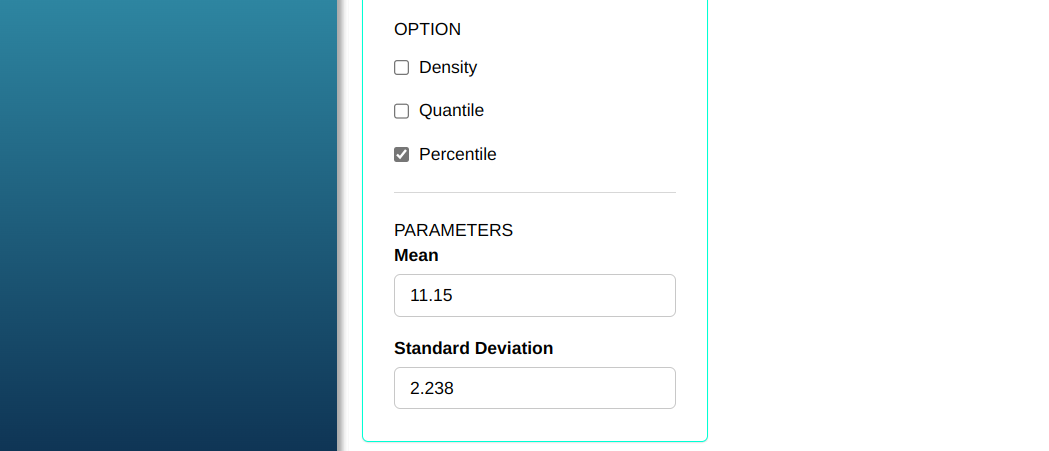
Consider X a Normal random variable with mean 11.15 and deviation standard 2.238. Let’s calculate certain percentiles of this distribution.
| V1 |
|---|
| 7.57 |
| 12.29 |
| 10.35 |
| 16.28 |
| 11.79 |
| 10.17 |
| 10.77 |
| 11.27 |
| 7.39 |
| 8.25 |
| 8.39 |
| 12.27 |
| 12.82 |
| 12.26 |
| 12.07 |
| 9.72 |
| 8.45 |
| 8.67 |
| 11.17 |
| 8.4 |
| 11.92 |
| 9.39 |
| 9.62 |
| 18.53 |
| 11.67 |
| 8.75 |
| 9.63 |
| 13.06 |
| 4.69 |
| 12.43 |
| 7.69 |
| 10.64 |
| 10.55 |
| 8.85 |
| 6.02 |
| 8.88 |
| 15.46 |
| 12.79 |
| 11.27 |
| 8.01 |
| 9.69 |
| 9.91 |
| 8.43 |
| 12.88 |
| 11.5 |
| 9.82 |
| 14.55 |
| 9.88 |
| 13.25 |
| 10.35 |
We will upload the data to the system.
To calculate the percentiles, the following configuration is performed, as shown in the following figure.

Then click Calculate to get the results. You can also generate the analyses and download them in Word format.
The results are as follows:
| Results |
|---|
| 0.055 |
| 0.695 |
| 0.360 |
| 0.989 |
| 0.612 |
| 0.331 |
| 0.432 |
| 0.522 |
| 0.047 |
| 0.097 |
| 0.109 |
| 0.692 |
| 0.772 |
| 0.691 |
| 0.659 |
| 0.262 |
| 0.114 |
| 0.134 |
| 0.504 |
| 0.109 |
| 0.634 |
| 0.215 |
| 0.247 |
| 1,000 |
| 0.591 |
| 0.142 |
| 0.248 |
| 0.804 |
| 0.002 |
| 0.716 |
| 0.061 |
| 0.411 |
| 0.394 |
| 0.152 |
| 0.011 |
| 0.155 |
| 0.973 |
| 0.768 |
| 0.521 |
| 0.080 |
| 0.257 |
| 0.289 |
| 0.112 |
| 0.780 |
| 0.562 |
| 0.277 |
| 0.936 |
| 0.285 |
| 0.826 |
| 0.360 |
Example 3:
Consider X a Normal random variable with mean 11.15 and deviation standard 2.238. Let’s calculate certain quantiles of this distribution.
First, let’s type the probabilities for which we want to find the quantiles of the distribution of interest.
We will upload the data to the system.

To calculate the quantiles, the following configuration is performed, as shown in the following figure.
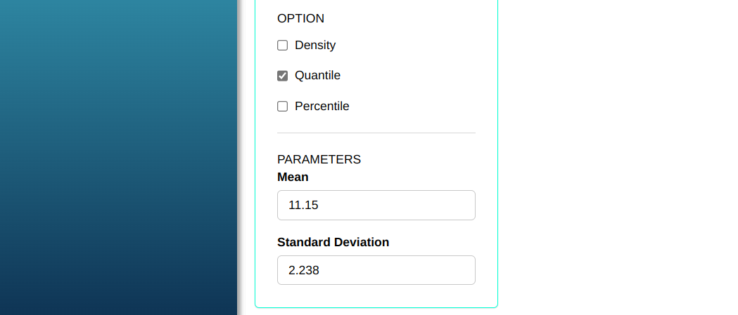
Then click Calculate to get the results. You can also generate the analyses and download them in Word format.
The results are as follows:
| Results |
|---|
| 12.32361 |
| 13.03355 |
| 14.01811 |
| 14.83118 |
Example 4:
Suppose that in a production line the probability of obtaining a part defective (success) is p=0.1. A sample of 4 pieces is taken to be inspected. What is the probability of obtaining a defective part, no defective parts, 2 defective parts, 3 and 4 defective parts?
First, let’s type the possible values that the variable random can assume, in this case it would be the quantity of pieces that can be defective
To calculate the probability density, the following setup is performed as shown in the following figure.

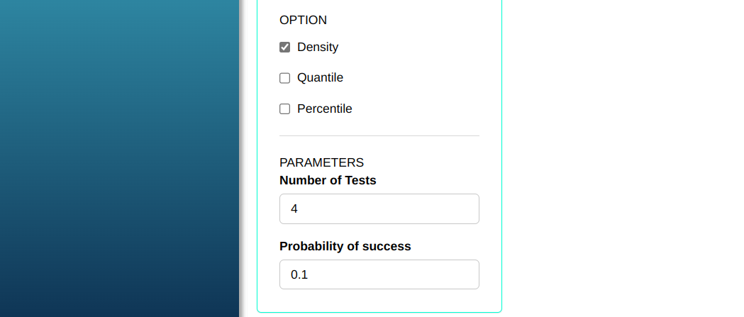
Then click Calculate to get the results. You can also generate the analyses and download them in Word format.
The results are as follows:
| Results |
|---|
| 0.6561 |
| 0.2916 |
| 0.0486 |
| 0.0036 |
| 0.0001 |
From the table, we see that the probabilities of obtaining a defective part is 29.16%, no defective parts is 65.61%, and obtaining two defective parts is 4.86% and for more than two it is less than 1%
Example 5:
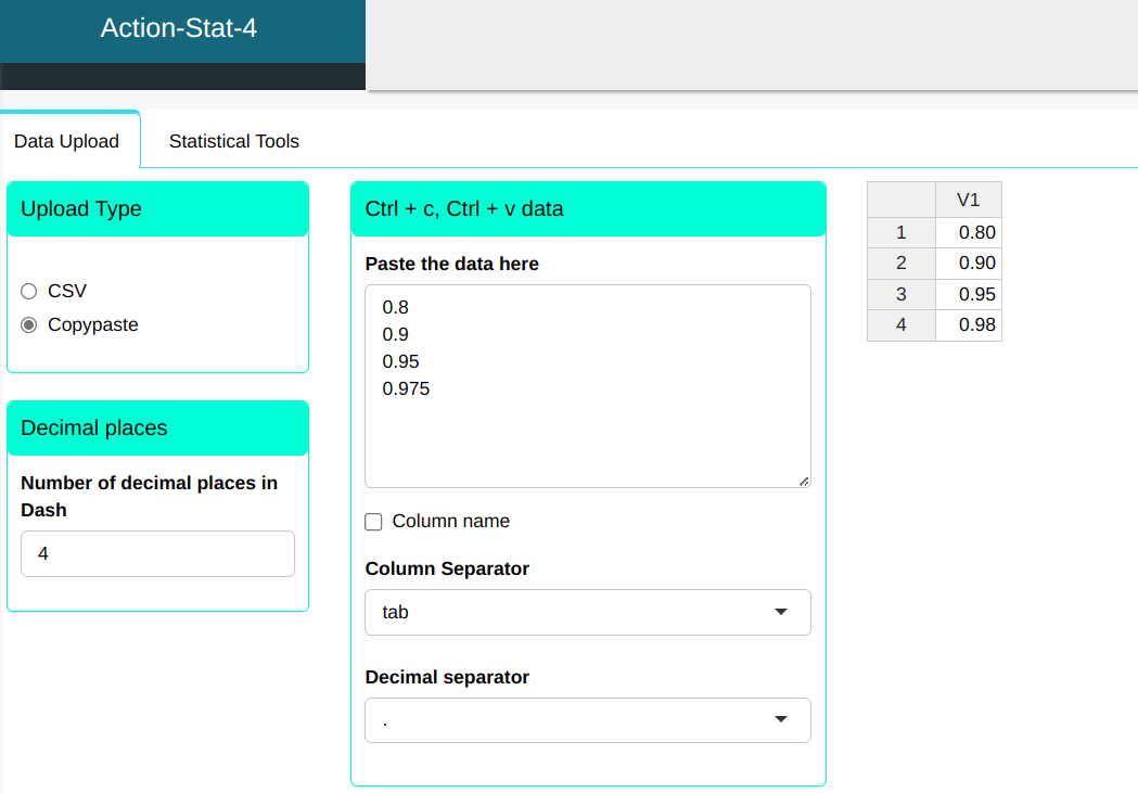
Consider a random variable X with Binomial distribution with parameters n=10 and prob=0.1. Calculate the quantile of X being less than 0.8 (80%), 0.9 (90%), 0.95 (95%) and 0.975 (97.5%).
First, let’s type the probabilities we want find the quantiles of the distribution of interest
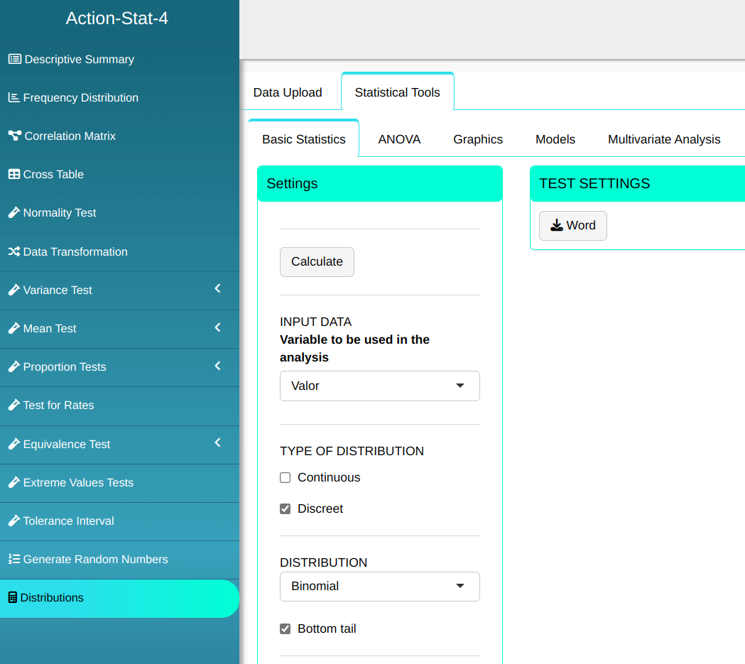
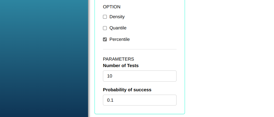
To calculate the quantiles, the following configuration is performed, as shown in the following figure.


Then click Calculate to get the results. You can also generate the analyses and download them in Word format.
The results are as follows:
| Results |
|---|
| 2 |
| 2 |
| 3 |
| 3 |
If the process is a 10 attempts experiment with a 10% probability of success
- In 80% of cases, we observe at most 2 successes.
- In 90% of cases, we observe at most 2 successes.
- In 95% of cases, we observe at most 3 successes.
- In 97.5% of cases, we observe at most 3 successes.
Example 6:
Suppose that in a production line the probability of obtaining a part defective (success) is p=0.1. A sample of 10 pieces is taken to be inspected. What is the probability of obtaining 3 defects or less?
First, let’s type the value at which we will calculate the percentile
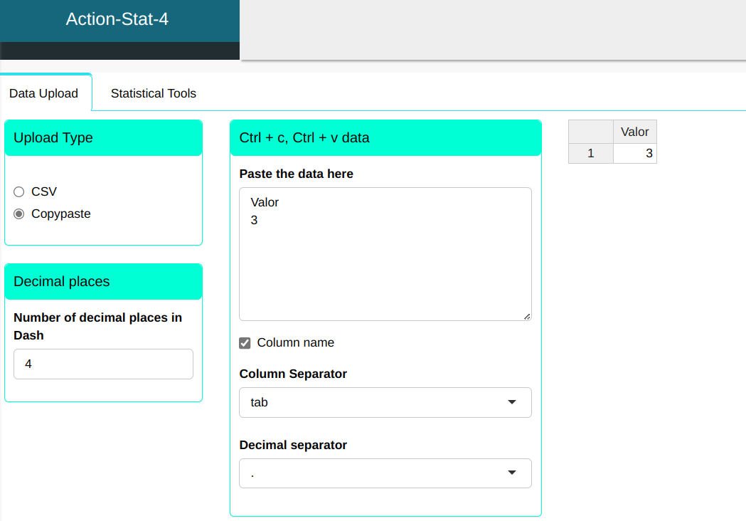
To calculate the percentiles, the following configuration is performed, as shown in the following figure.
Then click Calculate to get the results. You can also generate the analyses and download them in Word format.
The results are as follows:
| vetNum |
|---|
| 0.9872048 |
Based on the released value, we have the probability of obtaining 3 defects or less is approximately 98.72%.