1. Descriptive summary
Initial stage of an analysis, used to describe, organize and summarize the important aspects of the data collected.
Details
The descriptive summary allows us to obtain various information about the data set: minimum, maximum, sum, quadratic sum, size of sample, 1st quartile, 3rd quartile and tri-mean. In addition to this information, it is possible to calculate measures of position (mean and median), measures of dispersion (standard deviation of the mean, standard deviation, variance and amplitude) and other descriptive statistics such as asymmetry and kurtosis.
Example 1:
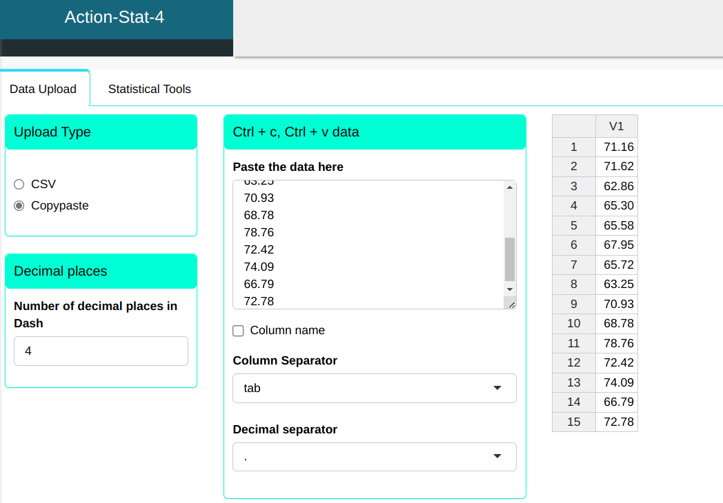
The length measurement of 15 rolls of steel has been taken and we will upload it in the system:
| 71.16 |
| 71.62 |
| 62.86 |
| 65.30 |
| 65.58 |
| 67.95 |
| 65.72 |
| 63.25 |
| 70.93 |
| 68.78 |
| 78.76 |
| 72.42 |
| 74.09 |
| 66.79 |
| 72.78 |
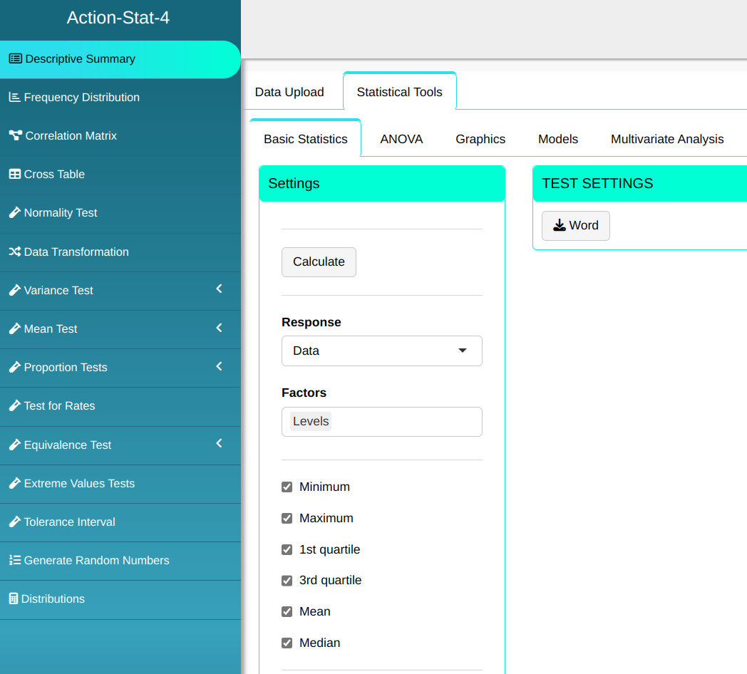
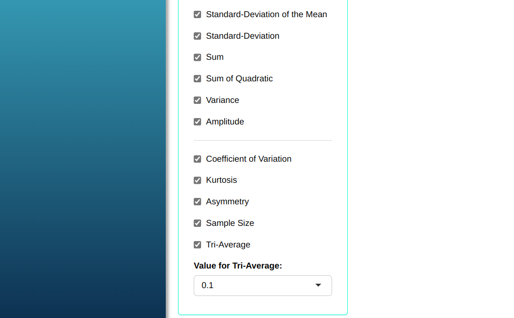
The descriptive summary is prepared according to the configuration shown in the figure below.
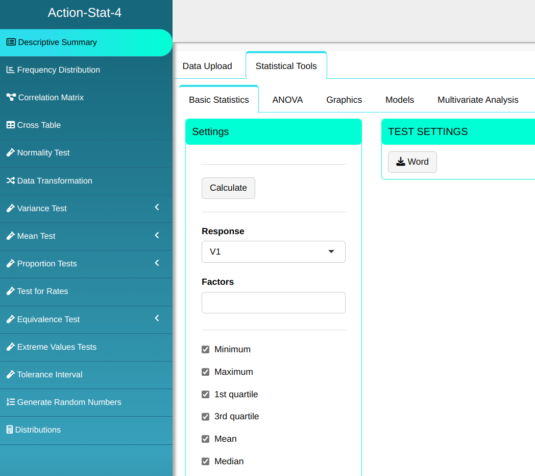
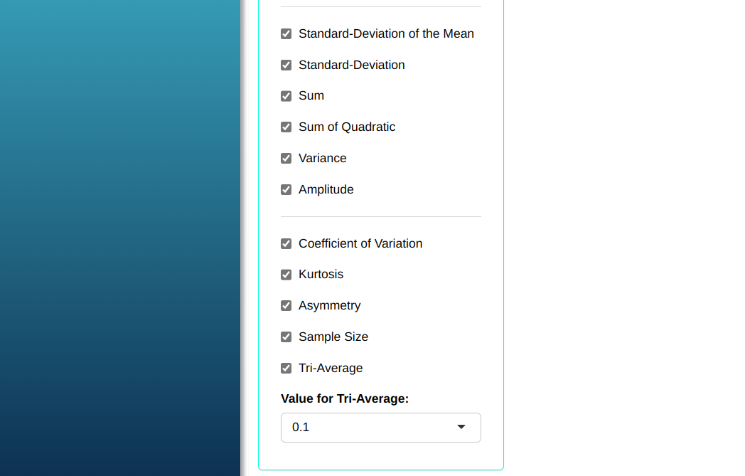
Then click Calculate view the results. You can also download them in a Word document.

We obtain the following results:
| Descriptive | Statistics |
|---|---|
| Minimum: | 62.86 |
| 1st quartile: | 65.58 |
| Average: | 69.199333 |
| Median: | 68.78 |
| Triaverage: | 68.951538 |
| 3rd quartile: | 72.42 |
| Maximum: | 78.76 |
| Sum: | 1,037.99 |
| Quadratic sum: | 72102.9673 |
| Standard deviation of the mean: | 1.1438267 |
| Standard deviation: | 4.430022 |
| Variation: | 19.625092 |
| Coefficient of variation: | 6.401827 |
| Skewness: | 0.358057 |
| Kurtosis: | -0.799861 |
| Amplitude: | 15,900 |
| Sample size: | 15 |
The mean and median are representatives of the overall distribution of the length of the rolls of wire in the sample.
-
The resulting variability is considerable if the lengths of the wire rolls are to be close. This can be seen from the dispersion measurements.
-
The distribution function is flatter than the Normal distribution, because the Kurtosis is less than zero. As the Asymmetry value is positive, but a small value, the distribution function has a slightly longer tail on the right, i.e. the distribution is asymmetric to the right.
-
Both the mean and the median can be considered representative of the general distribution of the sample data since both have close values. However, when the median value is very different from the mean, It is advisable to always consider the median as the most reference value. important.
Example 2:
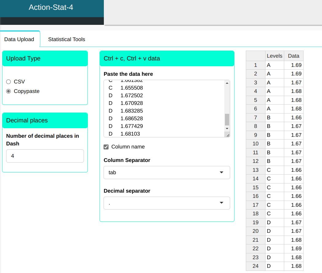
The diameter of the piece was measured by four operators, A, B, C and D, under the same conditions. 6 piece were chosen at random and the measurements obtained are shown in the following table. In this case we have a data set with a single factor, Operators, and four levels, Operator A, Operator B, Operator C and Operator D.
| Levels | Data |
|---|---|
| A | 1.688109 |
| A | 1.685566 |
| A | 1.672408 |
| A | 1.680943 |
| A | 1.679250 |
| A | 1.682141 |
| B | 1.663774 |
| B | 1.665943 |
| B | 1.669364 |
| B | 1.671857 |
| B | 1.665928 |
| B | 1.670507 |
| C | 1.658883 |
| C | 1.660408 |
| C | 1.663021 |
| C | 1.662004 |
| C | 1.661382 |
| C | 1.655508 |
| D | 1.672502 |
| D | 1.670928 |
| D | 1.683285 |
| D | 1.686528 |
| D | 1.677429 |
| D | 1.681030 |
Next we will make the descriptive summary.
The descriptive summary is prepared according to the configuration shown in the figure below.
Then click Calculate to get the results. You can also generate the analyses and download them in Word format.
We obtain the following results:
| Levels | A | B | C | D |
|---|---|---|---|---|
| Minimum | 1.672408 | 1.663774 | 1.655508 | 1.670928 |
| 1st quartile | 1.6775395 | 1.6653895 | 1.65803925 | 1.67221085 |
| Average | 1.6814028 | 1.6678955 | 1.660201 | 1.678617 |
| Medium | 1.681542 | 1.6676535 | 1.660895 | 1.6792295 |
| Triaverage | 1.6814028 | 1.6678955 | 1.660201 | 1.678617 |
| 3rd quartile | 1.68620175 | 1.6708445 | 1.6622583 | 1.6840958 |
| Maximum | 1.688109 | 1.671857 | 1.663021 | 1.686528 |
| Sum | 10.088109 | 10.007373 | 9.961206 | 10.071702 |
| Quadratic sum | 16.96284153 | 16.69130173 | 16.53764056 | 16.90671831 |
| Standard deviation of the mean | 0.002225628 | 0.0012824453 | 0.00110154 | 0.00250414 |
| Standard deviation | 0.00545165 | 0.0031413367 | 0.00269823 | 0.006133873 |
| Variation | 0.00007972 | 0.00000987 | 0.00000728 | 0.00003762 |
| Variation coefficient | 0.32423250 | 0.188341338 | 0.16252422 | 0.36541231 |
| Asymmetry | -0.3740836 | -0.010343887 | -0.64230944 | -0.05347545 |
| Kurtosis | -1.3224643 | -1.94651104 | -1.22707584 | -1.90258576 |
| Amplitude | 0.015701 | 0.008083 | 0.007513 | 0.0156 |
| Sample size | 6 | 6 | 6 | 6 |
The means and medians for each level are represent of the overall distribution of the diameter of pieces measured by each of the operators.
-
The resulting variability is not significant.
-
The distribution function is flatter than the Normal distribution, as the Kurtosis is negative at all levels. As the Asymmetry value is also negative at all levels, the distribution function has a slightly longer tail on the left, i.e. the distribution is asymmetric to the left.