11. Equivalence Test
The Equivalence Test tool offers analysis for Continuous data with equal or different variances, and also offers non-inferiority, superiority and equivalence tests for binary data.
Example 1:
In this example, we want to test whether a new methodology is superior to the compendial methodology. To do this, the proportion of positive results for both methods is evaluated. The summarized data is given in the following table.
| Results | Alternative | Compendial |
|---|---|---|
| Positive | 133 | 105 |
| Sterile | 17 | 45 |
| Total | 150 | 150 |
We will upload the data to the system.


Then click Calculate to get the results. You can also generate the analyses and download them in Word format.

The results are as follows
This section is based on the United States Pharmacopeia norma [1], which defines the hypothesis of Superiority as the proportion of positive results for the alternative procedure (AP) minus the proportion of positive results for the traditional or compendial procedure (PC). positive results for the alternative procedure (AP) minus the proportion of positive results for the traditional or compendial procedure (CP), with a tolerance margin of Superiority (Delta = 0.2). The hypothesis of Superiority is given by:
$$H_0: Pa-Pc \leq \Delta$$
$$H_1: Pa-Pc > \Delta$$
| Symbol | Caption/Formula |
|---|---|
| Na | Sample Size of the Alternative Method |
| Nc | Sample Size of the Compendial |
| Xa | Amount of Positivation of the Alternative Method |
| Xc | Amount of Positivation of the Traditional Method |
| Pa | Proportion for Alternative Method |
| Pc | Proportion for the Compendial Method |
| ^Pa | Xa/Na |
| ^Pc | Xc/Nc |
| theta? | Nc/Na |
| R | Pa/Pc |
| a | 1+theta |
| b | -[R(1+theta ^Pc)+theta+^Pa] |
| c | R(^Pa+theta ^Pc) |
| ~Pa | (-b-raiz(b²-4ac))/2a |
| ~Pc | ~Pa/R |
| V | [~Pa(1-~Pa)]/Na+R²[~Pc(1-~Pc)]/Nc |
| Z | (^Pa-R^Pc)/raiz(V) |
$\quad$ Superiority Test Results
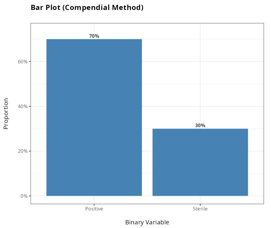
Compendial Method Results
| Quantity | Estimated Proportion | |
|---|---|---|
| Positive | 105 | 0.7 |
| Sterile | 45 | 0.3 |
| Total | 150 | 1.0 |
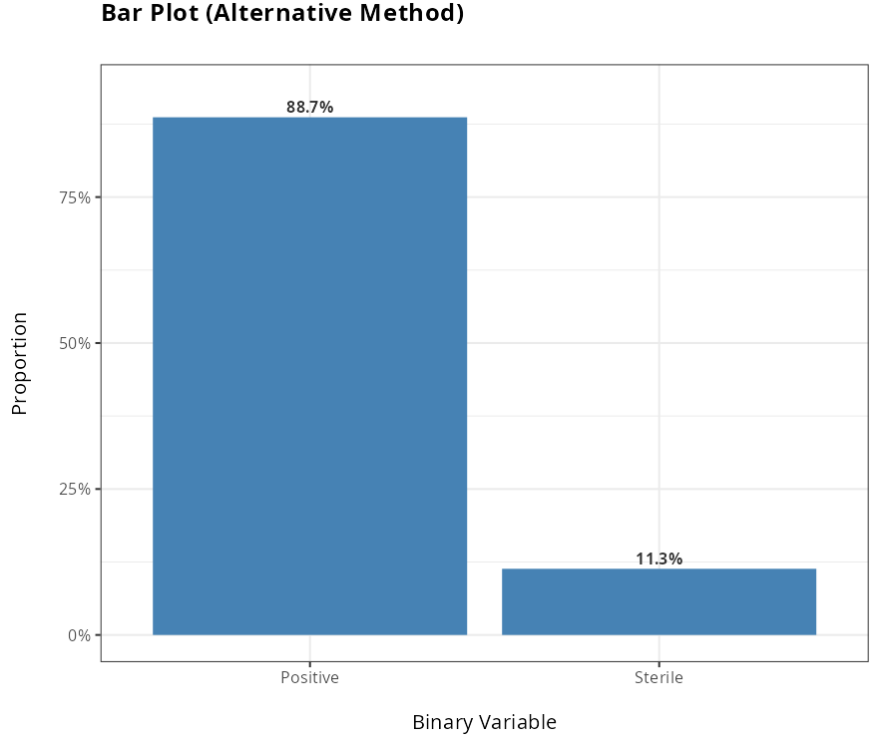
Alternative Method Results
| Quantity | Estimated Proportion | |
|---|---|---|
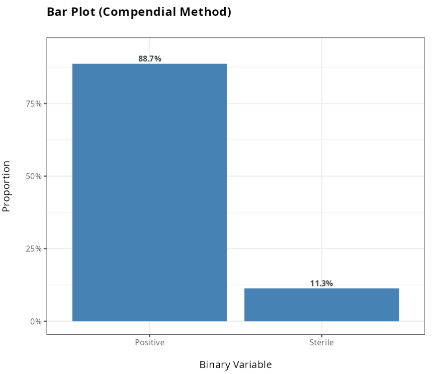
| Positive | 133 | 0.8866667 |
| Sterile | 17 | 0.1133333 |
| Total | 150 | 1.0000000 |
Test Parameters
$$H_0: Pa-Pc \leq \Delta$$
$$H_1: Pa-Pc > \Delta$$
| Value | |
|---|---|
| Theta | 1.000000000 |
| Proportions Ratio (R) | 1.400000000 |
| a | 2.000000000 |
| b | -4.266666667 |
| c | 2.221333333 |
| ~pa | 0.902012146 |
| ~pc | 0.644294390 |
| Variance (V) | 0.003583849 |
| Square Root (V) | 0.059865256 |
| ^pa-R*^pc | -0.093333333 |
| Z Statistics | -1.559056788 |
Rejection Criteria
| Value | |
|---|---|
| Significance level | 0.0500000 |
| Standardized Normal Quantiles - Superiority | 1.6448536 |
| P-Value | 0.9405085 |
Confidence Interval
| Value | |
|---|---|
| Confidence Level | 0.95 |
| Upper Limit | 0.261502 |
From the results obtained, we did not reject the null hypothesis at the 5% significance level. Therefore, we conclude that the Alternative method is not superior to the Traditional method.
Example 2:
In this example we want to test whether a new methodology is equivalent to the compendial methodology. To do this, we evaluate the proportion of positive results for both methods. The summarized data are given in the following Table
| Results | Alternative | Compendial |
|---|---|---|
| Positive | 105 | 133 |
| Sterile | 45 | 17 |
| Total | 150 | 150 |
We will upload the data to the system.


Then click Calculate to get the results. You can also generate the analyses and download them in Word format.
The results are as follows
This section is based on the United States Pharmacopeia norm [1], which defines the Equivalence hypothesis as the proportion of positive results for the alternative procedure (AP) minus the proportion of positive results for the traditional or compendial procedure (PC), with an Equivalence tolerance margin (Delta = -0.2). The Equivalence hypothesis is given by:
$$H_0: Pa-Pc \leq -\Delta \quad \textrm{or} \quad Pa-Pc \geq \Delta$$
$$H_1: -\Delta < Pa-Pc < \Delta$$
| Symbol | Caption/Formula |
|---|---|
| Na | Sample Size of the Alternative Method |
| Nc | Sample Size of the Compendial |
| Xa | Amount of Positivation of the Alternative Method |
| Xc | Amount of Positivation of the Traditional Method |
| Pa | Proportion for Alternative Method |
| Pc | Proportion for the Compendial Method |
| ^Pa | Xa/Na |
| ^Pc | Xc/Nc |
| theta? | Nc/Na |
| R | Pa/Pc |
| a | 1+theta |
| b | -[R(1+theta ^Pc)+theta+^Pa] |
| c | R(^Pa+theta ^Pc) |
| ~Pa | (-b-raiz(b²-4ac))/2a |
| ~Pc | ~Pa/R |
| V | [~Pa(1-~Pa)]/Na+R²[~Pc(1-~Pc)]/Nc |
| Z | (^Pa-R^Pc)/raiz(V) |
$\quad$ Equivalence Test Results
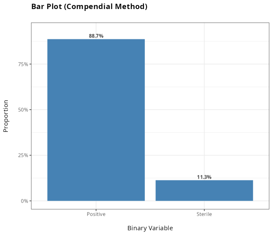
Compendial Method Results
| Quantity | Estimated Proportion | |
|---|---|---|
| Positive | 133 | 0.8866667 |
| Sterile | 17 | 0.1133333 |
| Total | 150 | 1.0000000 |
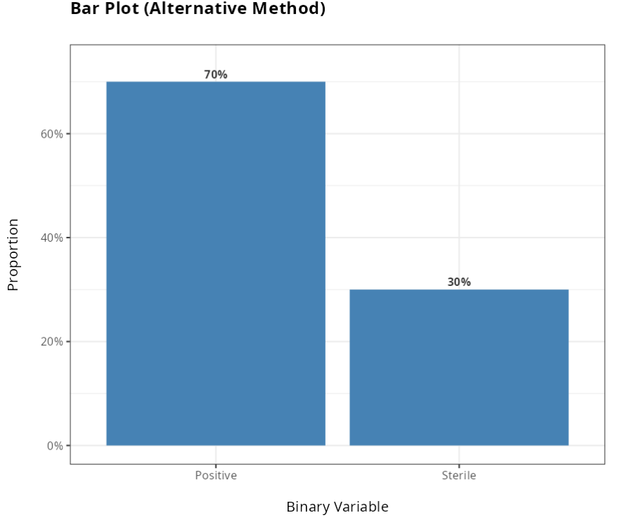
Alternative Method Results
| Quantity | Estimated Proportion | |
|---|---|---|
| Positive | 105 | 0.7 |
| Sterile | 45 | 0.3 |
| Total | 150 | 1.0 |
Test Parameters
$$H_{01}: Pa-Pc \leq - \Delta$$
$$H_{11}: Pa-Pc > - \Delta$$
| Value | |
|---|---|
| Theta | 1.000000000 |
| Proportions Ratio (R) | 0.714285714 |
| a | 2.000000000 |
| b | -3.047619048 |
| c | 1.133333333 |
| ~pa | 0.644294390 |
| ~pc | 0.902012146 |
| Variance (V) | 0.001828494 |
| Square Root (V) | 0.042760897 |
| ^pa-R*^pc | 0.066666667 |
| Z Statistics | 1.559056788 |
Testing parameters
$$H_{01}: Pa-Pc \geq \Delta$$
$$H_{11}: Pa-Pc < \Delta$$
| Value | |
|---|---|
| Theta | 1.000000000 |
| Proportions Ratio (R) | 1.400000000 |
| a | 2.000000000 |
| b | -4.341333333 |
| c | 2.221333333 |
| ~pa | 0.825946021 |
| ~pc | 0.589961444 |
| Variance (V) | 0.004119312 |
| Square Root (V) | 0.064181866 |
| ^pa-R*^pc | -0.541333333 |
| Z Statistics | -8.434365747 |
Rejection Criteria
| Value | |
|---|---|
| Significance level | 0.05000000 |
| Standardized Normal Quantiles - No inferiority | 1.64485363 |
| Standardized Normal Quantiles - Superiority | -1.64485363 |
| P-Value | 0.05949147 |
Confidence Interval
| Value | |
|---|---|
| Confidence Level | 0.95 |
| Lower Limit | -0.26150165 |
| Upper Limit | -0.11183168 |
From the results obtained, we did not reject the null hypothesis at the 5% significance level. We therefore conclude that the Alternative method is not equivalent to the Traditional method.
Example 3:
Neste exemplo deseja-se testar se uma nova metodologia é não inferior a metodologia compendial. Para isso, avalia-se a proporção de resultados positivos para ambos os métodos. Os dados resumidos sao dados na Tabela a seguir.
| Results | Alternative | Compendial |
|---|---|---|
| Positive | 105 | 133 |
| Steril | 45 | 17 |
| Total | 150 | 150 |
We will upload the data to the system.


Then click Calculate to get the results. You can also generate the analyses and download them in Word format.
The results are as follows
This section is based on the United States Pharmacopeia norm [1], which defines the hypothesis of Non-Inferiority as the proportion of positive results for the alternative procedure (AP) minus the proportion of positive results for the traditional or compendial procedure (CP), with a tolerance margin of Non-Inferiority (Delta = -0.2). The hypothesis of Non-Inferiority is given by:
$$H_0: Pa-Pc \leq -\Delta$$ and $$H_1: Pa-Pc > -\Delta$$
| Symbol | Caption/Formula |
|---|---|
| Na | Sample Size of the Alternative Method |
| Nc | Sample Size of the Compendial |
| Xa | Amount of Positivation of the Alternative Method |
| Xc | Amount of Positivation of the Traditional Method |
| Pa | Proportion for Alternative Method |
| Pc | Proportion for the Compendial Method |
| ^Pa | Xa/Na |
| ^Pc | Xc/Nc |
| theta? | Nc/Na |
| R | Pa/Pc |
| a | 1+theta |
| b | -[R(1+theta ^Pc)+theta+^Pa] |
| c | R(^Pa+theta ^Pc) |
| ~Pa | (-b-raiz(b²-4ac))/2a |
| ~Pc | ~Pa/R |
| V | [~Pa(1-~Pa)]/Na+R²[~Pc(1-~Pc)]/Nc |
| Z | (^Pa-R^Pc)/raiz(V) |
$\quad$ Results of the Non-Inferiority Test
Compendial Method Results
| Quantity | Estimated Proportion | |
|---|---|---|
| Positive | 133 | 0.8866667 |
| Sterile | 17 | 0.1133333 |
| Total | 150 | 1.0000000 |
Alternative Method Results
| Quantity | Estimated Proportion | |
|---|---|---|
| Positive | 105 | 0.7 |
| Sterile | 45 | 0.3 |
| Total | 150 | 1.0 |
Test Parameters
$$H_0: Pa-Pc \leq -\Delta$$
$$H_1: Pa-Pc > -\Delta$$
| Value | |
|---|---|
| Theta | 1.000000000 |
| Proportions Ratio (R) | 0.714285714 |
| a | 2.000000000 |
| b | -3.047619048 |
| c | 1.133333333 |
| ~pa | 0.644294390 |
| ~pc | 0.902012146 |
| Variance (V) | 0.001828494 |
| Square Root (V) | 0.042760897 |
| ^pa-R*^pc | 0.066666667 |
| Z Statistics | 1.559056788 |
Rejection Criteria
| Value | |
|---|---|
| Significance Level | 0.05000000 |
| Standardized Normal Quantiles - No inferiority | 1.64485363 |
| P-Value | 0.05949147 |
Confidence Interval
| Value | |
|---|---|
| Confidence Level | 0.95 |
| Lower Limit | -0.26150165 |

Dos resultados obtidos, não rejeitamos a hipótese nula, ao nível de significância de 5%. Portanto, concluímos pela Inferioridade do método Alternativo em relação ao método Tradicional.
Example 4:
We are going to do the equivalence test for continuous data. We want to test the equivalence of two laboratories in the concentration of a particular drug, so we collected 10 drugs from each laboratory.
| Data | Factor |
|---|---|
| 100.5449 | A |
| 99.67155 | A |
| 99.32921 | A |
| 100.0855 | A |
| 100.2163 | A |
| 100.0495 | A |
| 100.0238 | A |
| 99.28651 | A |
| 100.1467 | A |
| 99.72407 | A |
| 102.0206 | C |
| 101.0006 | C |
| 101.8330 | C |
| 101.7111 | C |
| 101.7244 | C |
| 98.65855 | C |
| 100.3181 | C |
| 100.9711 | C |
| 99.16993 | C |
| 100.7830 | C |
We will upload the data to the system.
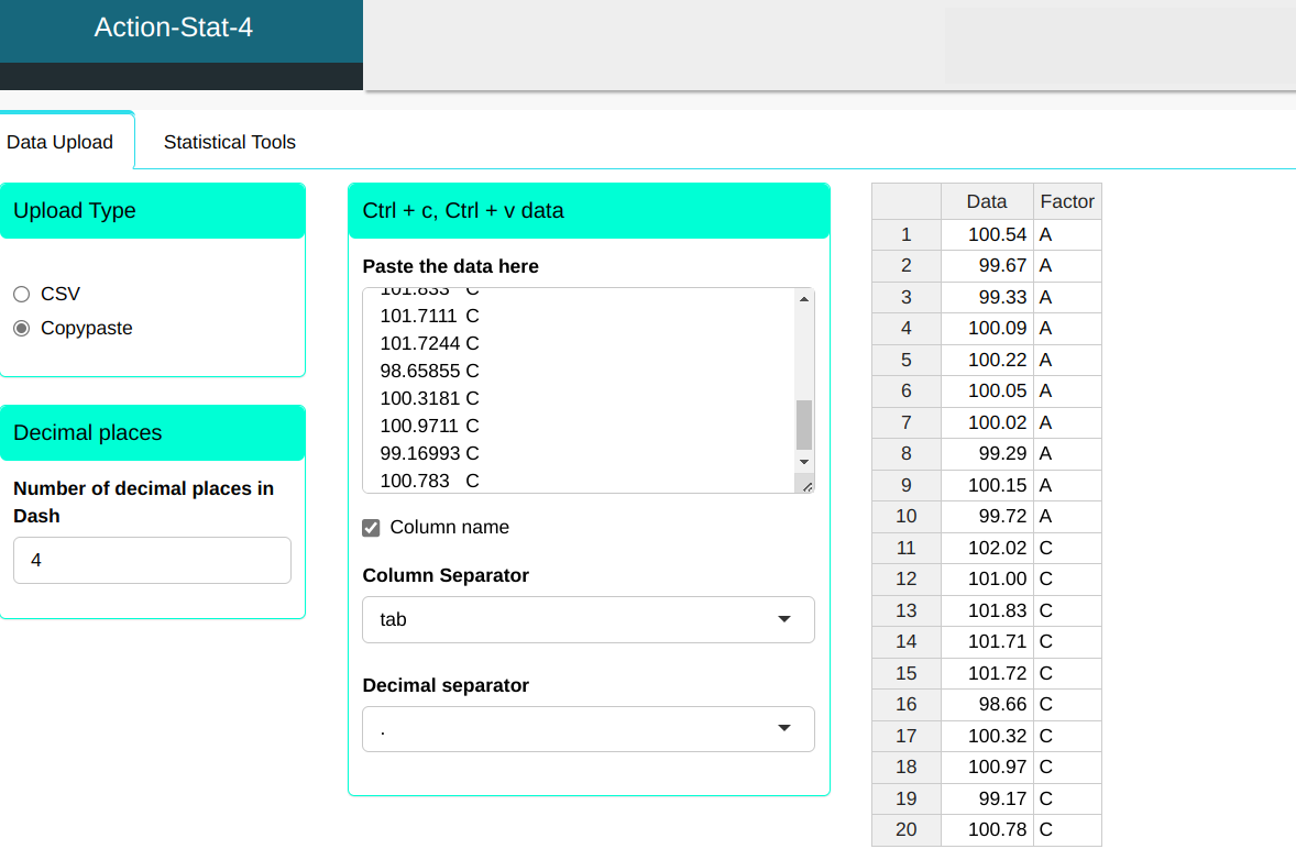
Configuring according to the figure below to make the test.


Then click Calculate to get the results. You can also generate the analyses and download them in Word format.
The results are as follows
Avaliação da Equivalência
To perform the equivalence test, we perform a t-test with the following hypotheses:
$$H_0: m1-m2 \leq -d \quad \textrm{or} \quad m1-m2 \geq d$$
$$H_1: -d < m1-m2 < d$$
As quais podem ser escritas como:
$$H_{01}: m1-m2 \leq -d \qquad \textrm{and} \qquad H_{11}: m1-m2 \geq -d$$ $$H_{02}: m1-m2 \geq d \qquad \textrm{and} \qquad H_{12}: m1-m2 < d$$
Results
| Values | |
|---|---|
| Degrees of Freedom | 11.1581 |
| P-value | 0.4107 |
| Mean - A | 99.9078 |
| Mean - C | 100.8190 |
| Standard Deviation - A | 0.3991 |
| Standard Deviation - C | 1.1442 |
| Sample Size - A | 10 |
| Sample Size - C | 10 |
| Confidence Level | 0.9500 |
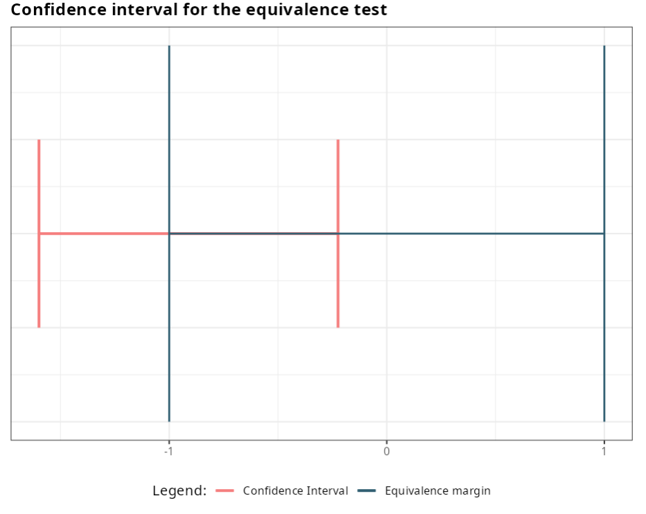
| Lower Limit | -1.5985 |
| Upper Limit | -0.2239 |
| Equivalence Margin | 1 |
| Test 1 Statistic - $H_{01}: m1-m2 \leq -d$ | 0.2316 |
| Test 2 Statistic - $H_{02}: m1-m2 \geq d$ | 4.9874 |
At a significance level of 0.05, we do not reject the null hypothesis, i.e. we conclude that the characteristics tested are not equivalent at a significance level of 5%.
The results of the Variance Test are shown in the table.
| Sample | Group |
|---|---|
| 100.5449 | A |
| 99.6716 | A |
| 99.3292 | A |
| 100.0855 | A |
| 100.2163 | A |
| 100.0495 | A |
| 100.0238 | A |
| 99.2865 | A |
| 100.1467 | A |
| 99.7241 | A |
| 102.0206 | C |
| 101.0006 | C |
| 101.8330 | C |
| 101.7111 | C |
| 101.7244 | C |
| 98.6586 | C |
| 100.3181 | C |
| 100.9711 | C |
| 99.1699 | C |
| 100.7830 | C |
Test for Two Variances
| Values | |
|---|---|
| F Statistics | 0.121667 |
| Degrees of freedom (Numerator) | 9 |
| Degrees of freedom (Denominator) | 9 |
| P-Value | 0.00436814 |
| Standard Deviation - A | 0.3991091 |
| Standard Deviation - C | 1.144208 |
| Sample Size for A | 10 |
| Sample Size for C | 10 |
| Alternative Hypothesis Different from | 1 |
| Confidence Intervals for the Variances ratio | 95% |
| Lower Limit | 0.03022037 |
| Upper Limit | 0.4898308 |
Next, we present the graph containing the confidence interval and the margin of equivalence.
For a significance level of 0.05 we reject the null hypothesis, i.e. we conclude that the variances are statistically different.
With P-value > $\alpha$, the null hypothesis is not rejected. Thus, it is concluded that the laboratories are not equivalent at the significance level $\alpha$ = 5%.