2. Proportions: two samples
The two-sample proportions test is used to compare the rate of success of the experiments.
Example 1:
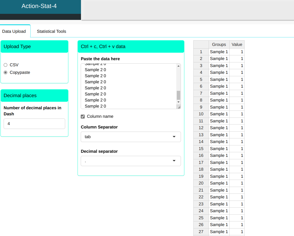
A company that provides economic advisory services to third parties. Companies are interested in comparing the rate of complaints about its services in two of its offices in two different cities. Suppose the company randomly selected 100 services. carried out by the city One office and 120 services carried out by city office B. The tables show these services (1 indicates that there was no complaint and 0 indicates that there was a complaint). the company wants know if these results are sufficient to conclude that the two offices present a significant difference between their complaints.
| Groups | Value |
|---|---|
| Sample 1 | 1 |
| Sample 1 | 1 |
| Sample 1 | 1 |
| Sample 1 | 1 |
| Sample 1 | 1 |
| Sample 1 | 1 |
| Sample 1 | 1 |
| Sample 1 | 1 |
| Sample 1 | 1 |
| Sample 1 | 1 |
| Sample 1 | 1 |
| Sample 1 | 1 |
| Sample 1 | 1 |
| Sample 1 | 1 |
| Sample 1 | 1 |
| Sample 1 | 1 |
| Sample 1 | 1 |
| Sample 1 | 1 |
| Sample 1 | 1 |
| Sample 1 | 1 |
| Sample 1 | 1 |
| Sample 1 | 1 |
| Sample 1 | 1 |
| Sample 1 | 1 |
| Sample 1 | 1 |
| Sample 1 | 1 |
| Sample 1 | 1 |
| Sample 1 | 1 |
| Sample 1 | 1 |
| Sample 1 | 1 |
| Sample 1 | 1 |
| Sample 1 | 1 |
| Sample 1 | 1 |
| Sample 1 | 1 |
| Sample 1 | 1 |
| Sample 1 | 1 |
| Sample 1 | 1 |
| Sample 1 | 1 |
| Sample 1 | 1 |
| Sample 1 | 1 |
| Sample 1 | 1 |
| Sample 1 | 1 |
| Sample 1 | 1 |
| Sample 1 | 1 |
| Sample 1 | 1 |
| Sample 1 | 1 |
| Sample 1 | 1 |
| Sample 1 | 1 |
| Sample 1 | 1 |
| Sample 1 | 1 |
| Sample 1 | 1 |
| Sample 1 | 1 |
| Sample 1 | 1 |
| Sample 1 | 1 |
| Sample 1 | 1 |
| Sample 1 | 1 |
| Sample 1 | 1 |
| Sample 1 | 1 |
| Sample 1 | 1 |
| Sample 1 | 1 |
| Sample 1 | 1 |
| Sample 1 | 1 |
| Sample 1 | 1 |
| Sample 1 | 1 |
| Sample 1 | 1 |
| Sample 1 | 1 |
| Sample 1 | 1 |
| Sample 1 | 1 |
| Sample 1 | 1 |
| Sample 1 | 1 |
| Sample 1 | 1 |
| Sample 1 | 1 |
| Sample 1 | 1 |
| Sample 1 | 1 |
| Sample 1 | 1 |
| Sample 1 | 1 |
| Sample 1 | 1 |
| Sample 1 | 1 |
| Sample 1 | 1 |
| Sample 1 | 1 |
| Sample 1 | 1 |
| Sample 1 | 1 |
| Sample 1 | 1 |
| Sample 1 | 1 |
| Sample 1 | 1 |
| Sample 1 | 1 |
| Sample 1 | 1 |
| Sample 1 | 1 |
| Sample 1 | 0 |
| Sample 1 | 0 |
| Sample 1 | 0 |
| Sample 1 | 0 |
| Sample 1 | 0 |
| Sample 1 | 0 |
| Sample 1 | 0 |
| Sample 1 | 0 |
| Sample 1 | 0 |
| Sample 1 | 0 |
| Sample 1 | 0 |
| Sample 1 | 0 |
| Sample 2 | 1 |
| Sample 2 | 1 |
| Sample 2 | 1 |
| Sample 2 | 1 |
| Sample 2 | 1 |
| Sample 2 | 1 |
| Sample 2 | 1 |
| Sample 2 | 1 |
| Sample 2 | 1 |
| Sample 2 | 1 |
| Sample 2 | 1 |
| Sample 2 | 1 |
| Sample 2 | 1 |
| Sample 2 | 1 |
| Sample 2 | 1 |
| Sample 2 | 1 |
| Sample 2 | 1 |
| Sample 2 | 1 |
| Sample 2 | 1 |
| Sample 2 | 1 |
| Sample 2 | 1 |
| Sample 2 | 1 |
| Sample 2 | 1 |
| Sample 2 | 1 |
| Sample 2 | 1 |
| Sample 2 | 1 |
| Sample 2 | 1 |
| Sample 2 | 1 |
| Sample 2 | 1 |
| Sample 2 | 1 |
| Sample 2 | 1 |
| Sample 2 | 1 |
| Sample 2 | 1 |
| Sample 2 | 1 |
| Sample 2 | 1 |
| Sample 2 | 1 |
| Sample 2 | 1 |
| Sample 2 | 1 |
| Sample 2 | 1 |
| Sample 2 | 1 |
| Sample 2 | 1 |
| Sample 2 | 1 |
| Sample 2 | 1 |
| Sample 2 | 1 |
| Sample 2 | 1 |
| Sample 2 | 1 |
| Sample 2 | 1 |
| Sample 2 | 1 |
| Sample 2 | 1 |
| Sample 2 | 1 |
| Sample 2 | 1 |
| Sample 2 | 1 |
| Sample 2 | 1 |
| Sample 2 | 1 |
| Sample 2 | 1 |
| Sample 2 | 1 |
| Sample 2 | 1 |
| Sample 2 | 1 |
| Sample 2 | 1 |
| Sample 2 | 1 |
| Sample 2 | 1 |
| Sample 2 | 1 |
| Sample 2 | 1 |
| Sample 2 | 1 |
| Sample 2 | 1 |
| Sample 2 | 1 |
| Sample 2 | 1 |
| Sample 2 | 1 |
| Sample 2 | 1 |
| Sample 2 | 1 |
| Sample 2 | 1 |
| Sample 2 | 1 |
| Sample 2 | 1 |
| Sample 2 | 1 |
| Sample 2 | 1 |
| Sample 2 | 1 |
| Sample 2 | 1 |
| Sample 2 | 1 |
| Sample 2 | 1 |
| Sample 2 | 1 |
| Sample 2 | 1 |
| Sample 2 | 1 |
| Sample 2 | 1 |
| Sample 2 | 1 |
| Sample 2 | 1 |
| Sample 2 | 1 |
| Sample 2 | 1 |
| Sample 2 | 1 |
| Sample 2 | 1 |
| Sample 2 | 1 |
| Sample 2 | 1 |
| Sample 2 | 1 |
| Sample 2 | 1 |
| Sample 2 | 1 |
| Sample 2 | 1 |
| Sample 2 | 1 |
| Sample 2 | 1 |
| Sample 2 | 1 |
| Sample 2 | 1 |
| Sample 2 | 1 |
| Sample 2 | 1 |
| Sample 2 | 1 |
| Sample 2 | 0 |
| Sample 2 | 0 |
| Sample 2 | 0 |
| Sample 2 | 0 |
| Sample 2 | 0 |
| Sample 2 | 0 |
| Sample 2 | 0 |
| Sample 2 | 0 |
| Sample 2 | 0 |
| Sample 2 | 0 |
| Sample 2 | 0 |
| Sample 2 | 0 |
| Sample 2 | 0 |
| Sample 2 | 0 |
| Sample 2 | 0 |
| Sample 2 | 0 |
| Sample 2 | 0 |
| Sample 2 | 0 |
We will upload the data to the system.
To perform the proportion test, the following configuration is made, which is shown in the following figure.
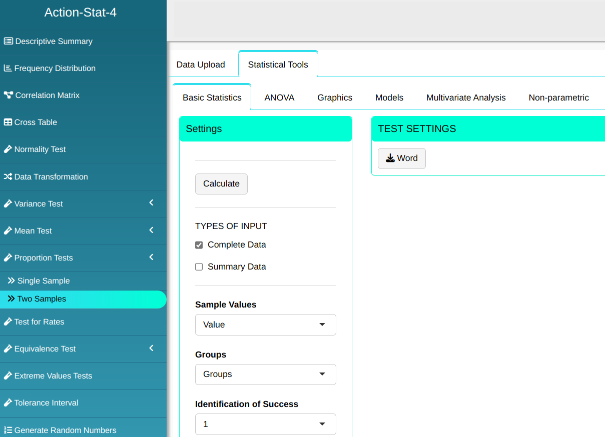

Then click Calculate to get the results. You can also generate the analyses and download them in Word format.

The results are as follows
Results - Sample 1
| Quantity | Proportions | |
|---|---|---|
| Success | 88 | 0.88 |
| Failure | 12 | 0.12 |
Results - Sample 2
| Quantity | Proportions | |
|---|---|---|
| Success | 102 | 0.85 |
| Failure | 18 | 0.15 |
Results - Normal approximation
| Values | |
|---|---|
| Z Statistics | 0.6456331 |
| P-value | 0.518517 |
| Proportion of Success in sample 1 | 0.88 |
| Proportion of Success in sample 2 | 0.85 |
| Alternative hypothesis | Different from 0 |
| Confidence level | 95% |
| Lower limit | -0.06021159 |
| Upper limit | 0.1202116 |
Since the p value obtained, 0.518517, is greater than the significance level adopted, of 0.05, so we do not reject the null hypothesis, of equality between proportions. Therefore, there is no evidence to say that the offices present a significant difference between their complaints.
Example 2:
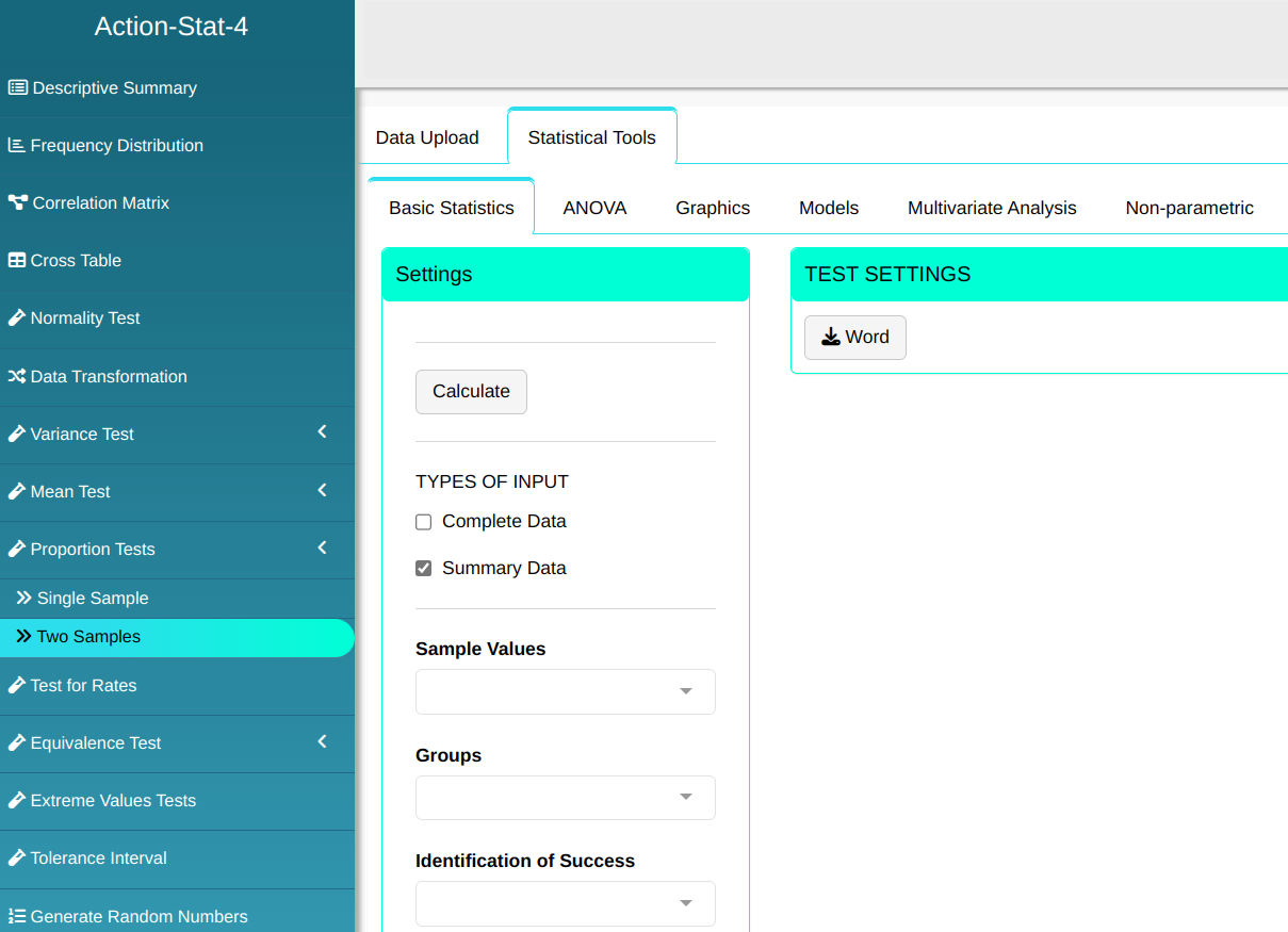
A company that provides economic advisory services to third parties. Companies are interested in comparing the rate of complaints about its services in two of its offices in two different cities. Suppose the company randomly selected 100 services. carried out by municipal office A and it was found that in 12 of them There was some kind of complaint. From the office in city B, 120 services were selected and 18 received some type of complaint. HE The company wants to know if these results are enough to conclude that the two offices present a significant difference among their complaint rates.
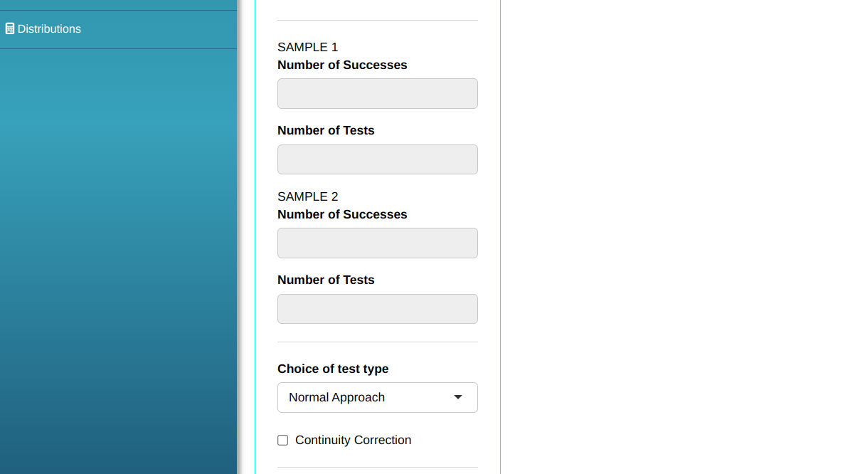
To perform the proportion test, the following configuration is made, which is shown in the following figure.
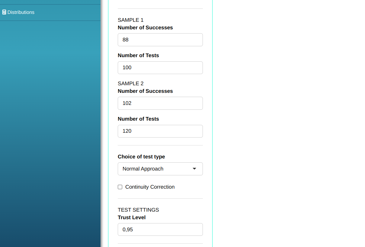

Then click Calculate to get the results. You can also generate the analyses and download them in Word format.
The results are as follows:
Results - Data set 1
| Quantity | Proportions | |
|---|---|---|
| Success | 88 | 0.88 |
| Failure | 12 | 0.12 |
Results - Data Set 2
| Quantity | Proportions | |
|---|---|---|
| Success | 102 | 0.85 |
| Failure | 18 | 0.15 |
Results - Normal approximation
| Values | |
|---|---|
| Z Statistics | 0.6456331 |
| P-value | 0.518517 |
| Success ratio in sample 1 | 0.88 |
| Success ratio in sample 2 | 0.85 |
| Alternative hypothesis | Different from 0 |
| Confidence level | 95% |
| Lower limit | -0.06021159 |
| Upper limit | 0.1202116 |
Since the p value obtained, 0.518517, is greater than the significance level adopted, of 0.05, so we do not reject the null hypothesis, of equality between proportions. Therefore, there is no evidence to say that the offices present a significant difference between their complaints.