6. Data Transformation

The Box-Cox transformation is one of the possible ways of solving problems for data that do not meet the assumptions of analysis of variance, such as data normality. analysis, such as data normality.

Example 1:

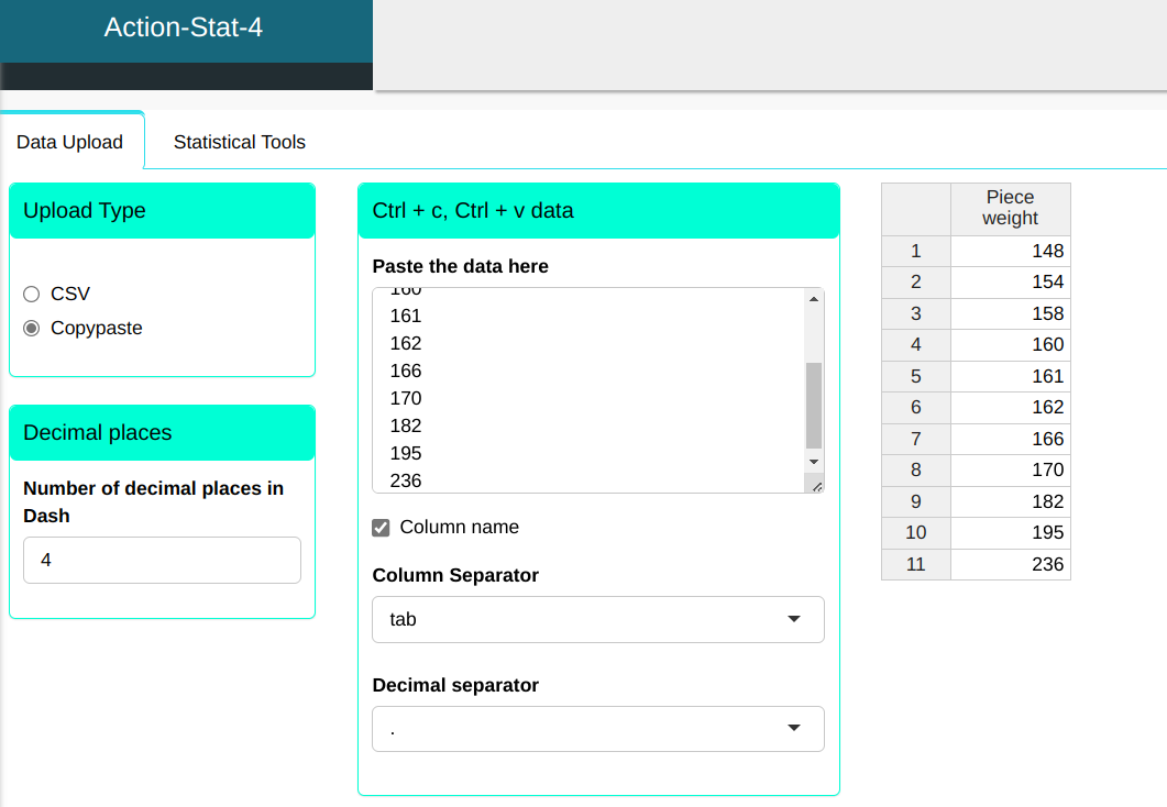
For a given analysis, the data must follow a normal distribution. distribution. One study found that the 11 measurements of piece weights (in pounds) did not follow this distribution. It is therefore necessary to use a transformation that circumvents the problem.

Piece weights
148
154
158
160
161
162
166
170
182
195
236

---

We will then upload it to the system.

---

Configuring as shown below to perform the data transformation.

---

---

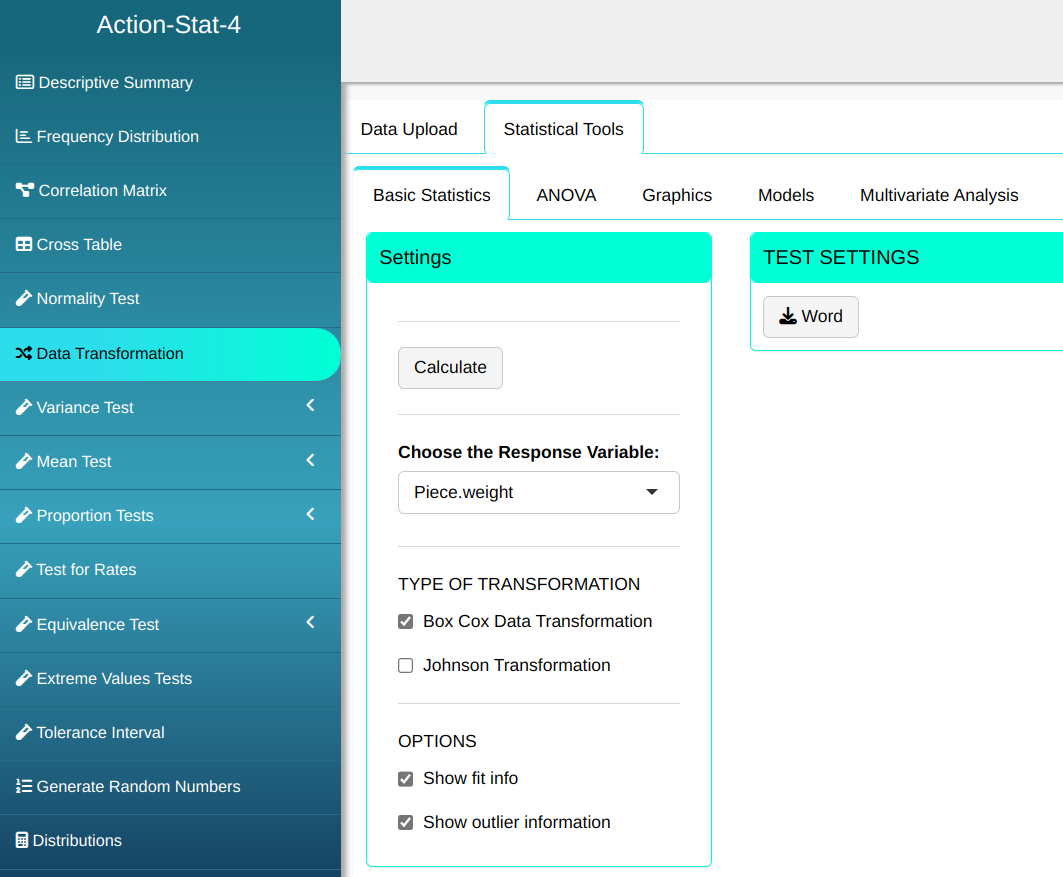
Then click Calculate to get the results. You can also generate the analyses and download them in Word format.

---

The results are as follows:

		Box-Cox Transformation

---

Results

	V1
Lambda	-2.500
P-Value (Anderson-Darling)	0.309

---

Transformed Data

Data1
0.4
0.4
0.4
0.4
0.4
0.4
0.4
0.4
0.4
0.4
0.4

---

Outliers (Quantiles)

Obs.	Normal Quantiles	Data	Criterion
11	$\qquad\qquad$ 1.69	0.4	Envelope (Confidence Level=95%)

---

---

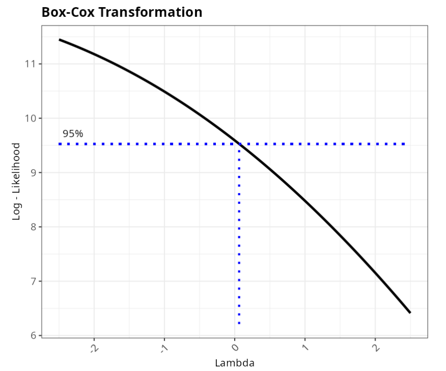
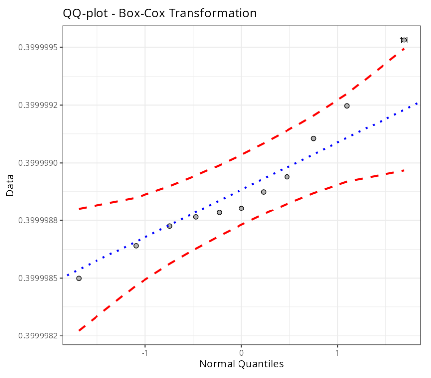
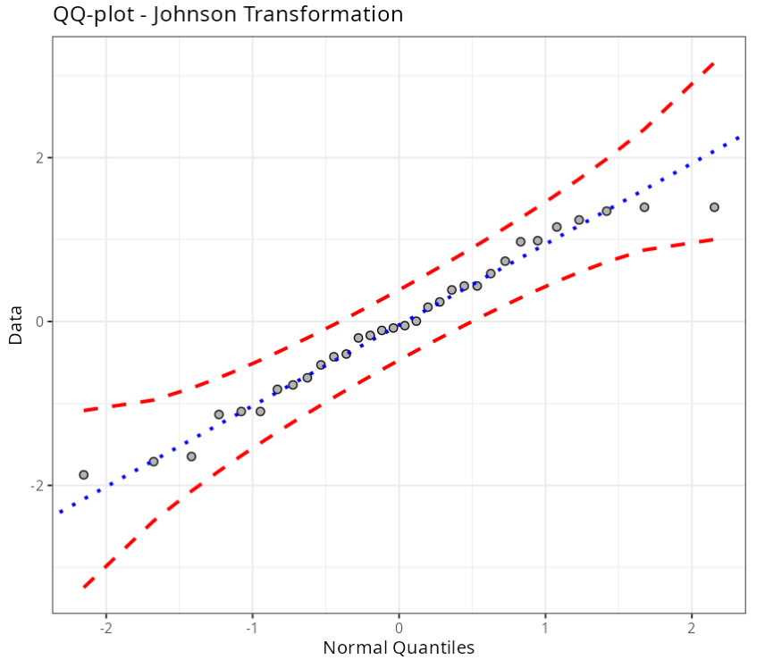
The QQ-plot shows that the assumption of normality is met, and we get a p-value of 0.309 in the Anderson-Darling test, which indicates that the data follows a normal distribution. We note that observation number 11 is outside the envelope of the QQ-plot, but this does not invalidate the assumption of normality of the transformed data.

Therefore, using the transformed data, it is possible to continue the study, since the assumption of normality of the data is met.

Example 2:

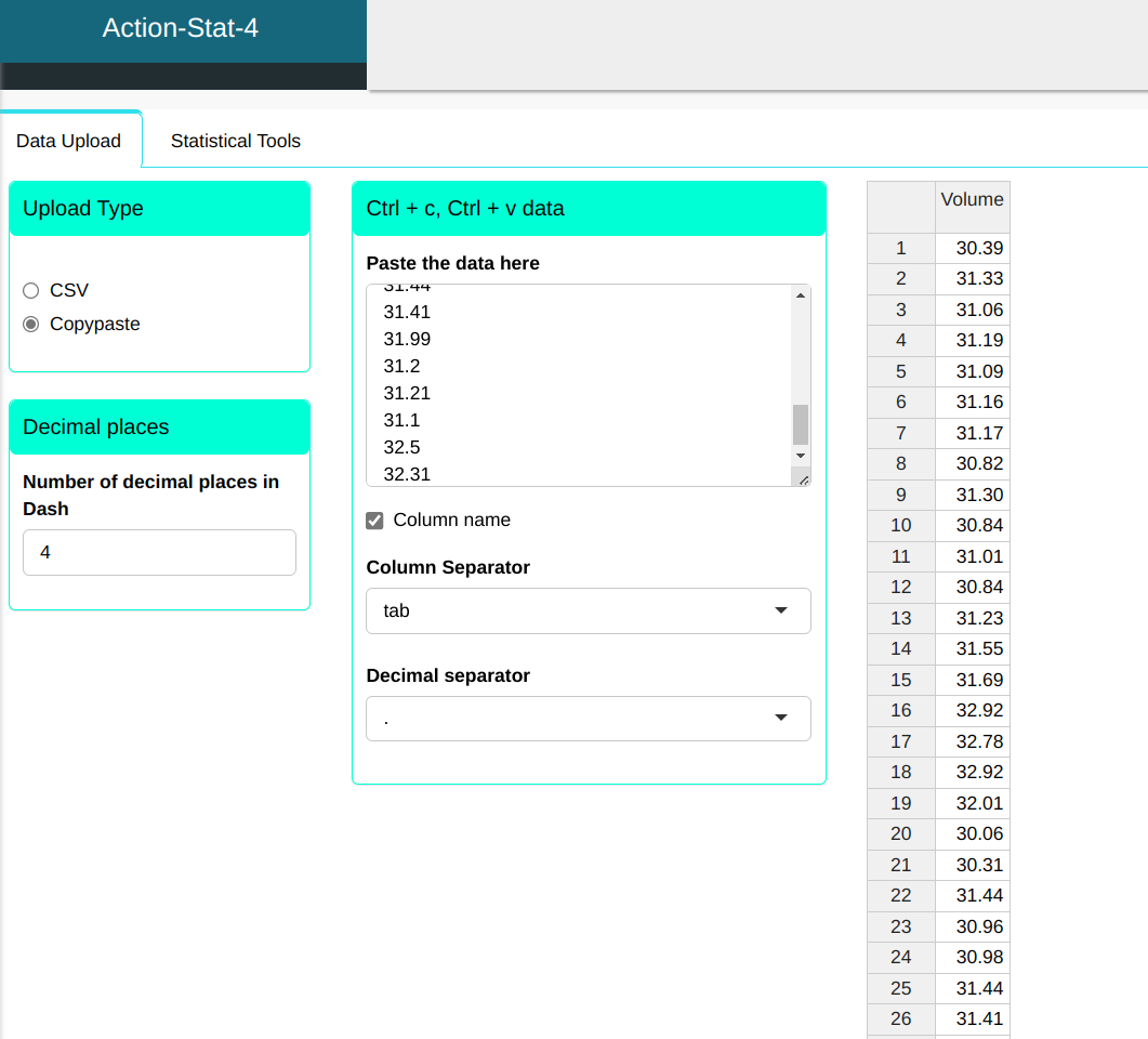
Consider a sample with 32 observations of the volume of a medicine bottle. The sample data does not have a normal distribution and we need to normalize the data in order to continue the study.

volume
30.39
31.33
31.06
31.19
31.09
31.16
31.17
30.82
31.3
30.84
31.01
30.84
31.23
31.55
31.69
32.92
32.78
32.92
32.01
30.06
30.31
31.44
30.96
30.98
31.44
31.41
31.99
31.2
31.21
31.1
32.5
32.31

---

We will upload the data to the system.

---

Configuring as shown below to perform the data transformation.

---

---

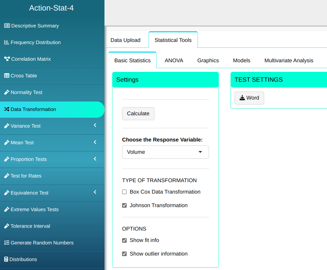
Then click Calculate to get the results. You can also generate the analyses and download them in Word format.

---

The results are as follows:

		Johnson Transformation

---

Estimates

	test
Gamma	-0.404546625366474
Lambda	0.178551759842957
Epsilon	31.0975476436831
Eta	0.596015901747296
Family	SU
P-Value (Anderson-Darling)	0.7745

---

Transformed Data

---

Data
-1.648
0.239
-0.529
-0.108
-0.430
-0.200
-0.169
-1.134
0.175
-1.097
-0.686
-1.097
0.005
0.585
0.737
1.395
1.347
1.395
0.986
-1.871
-1.710
0.434
-0.827
-0.773
0.434
0.386
0.974
-0.079
-0.050
-0.396
1.239
1.153

---