1. ID Plot

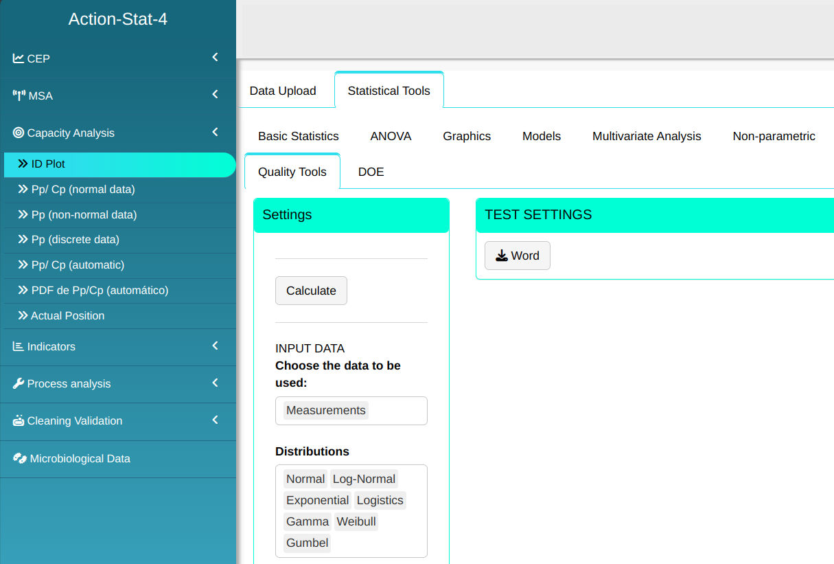
“ACTION” provides the ID-Plot tool allows you to determine which distribution best describes the randomness of a data set: Normal, Log-Normal, Exponential, Logistic, Gamma, Weibull e Gumbel. This tool allows you to choose between the QQPlot, Histogram, and Density Function graphs, as well as the Anderson-Darling, Cramer-von-Misses, and Kolmogorov-Smirnov hypothesis tests.

Example:

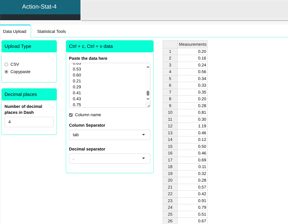
Consider the data set in the table below. Let’s see which probability distribution best describes this set of data.

Measurements
0.20
0.16
0.24
0.56
0.34
0.33
0.35
0.20
0.28
0.81
0.30
1.19
0.46
0.12
0.50
0.46
0.69
0.11
0.32
0.28
0.57
0.42
0.91
0.79
0.51
0.67
0.70
0.19
0.22
0.62
0.56
0.96
0.11
0.85
0.37
0.80
0.52
0.17
0.58
0.15
0.20
0.05
0.63
0.53
0.60
0.21
0.29
0.41
0.43
0.75

---

We will upload the data to the system.

Configuring as shown in the figure below to perform the analysis.

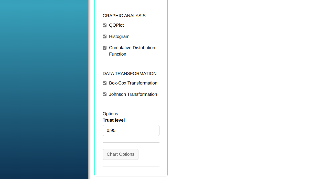
Then click Calculate to get the results. You can also generate the analyses and download them in Word format.

The results are:

Analysis result

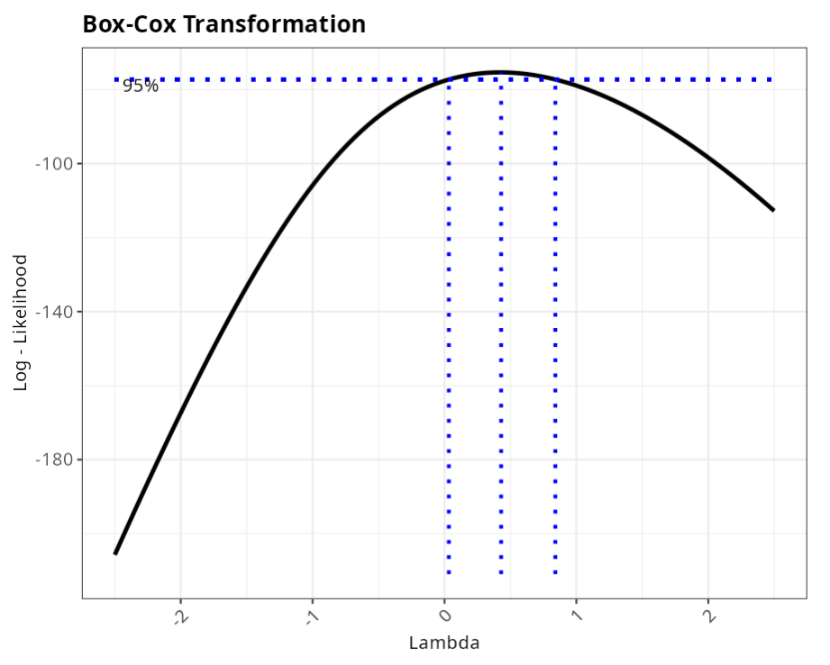
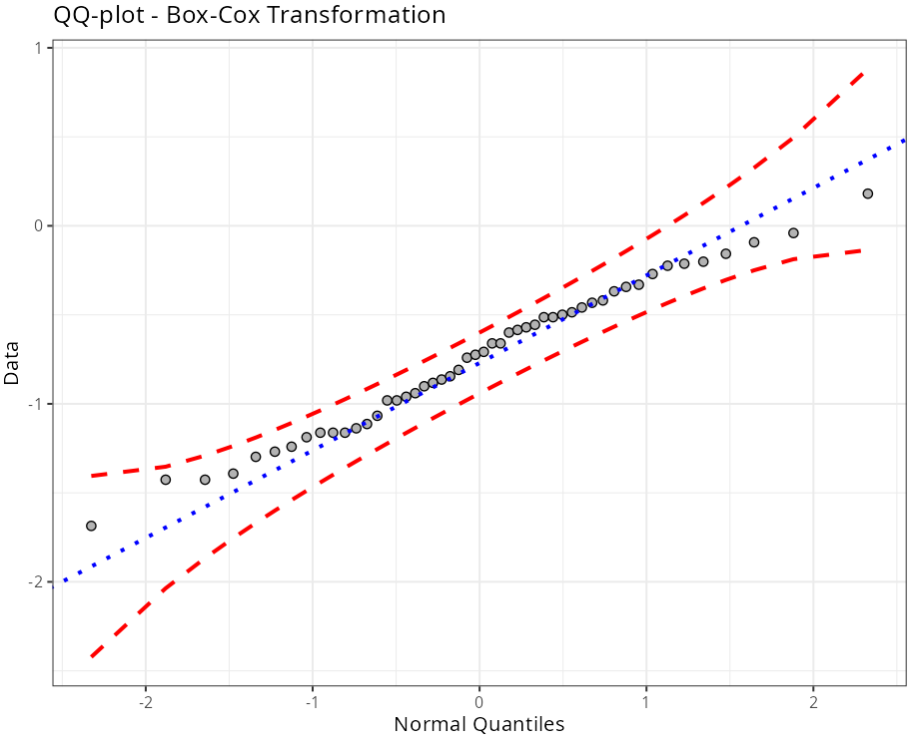
		Box-Cox Transformation

---

Results

	Valuess
Lambda	0.429
P-Value (Anderson-Darling)	0.703

---

Analysis result

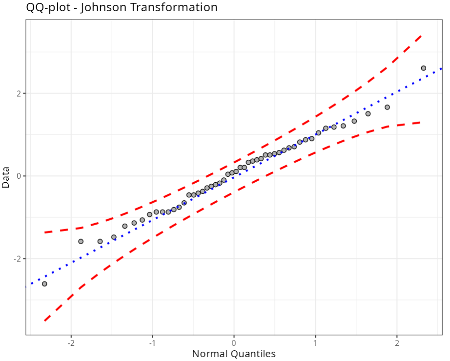
		Johnson TRAMSFORMATON

---

Estimates

	test
Gamma	0.90802942754439
Lambda	1.36936290670753
Epsilon	0.0168457063069285
Eta	0.951739827664239
Família	SB
P-Value (Anderson-Darling)	0.9422

---

Anderson-Darling

	Distributions	Statistics	P-Value
1	Normal($\mu$ = 0.45, $\sigma$ = 0.26)	0.566	0.136
2	Log-Normal(log($\mu$) = -0.982398, log($\sigma$)= 0.667801)	0.589	0.118
1-mle-exp	Exponentiall(Rate = 2.20556)	3.845	0.000
11	Logistica(Location = 0.44, Scale = 0.15)	0.581	0.089
12	Gamma(Shape = 2.76743, Rate = 6.10372)	0.295	0.250
13	Weibull(Shape = 1.84755, Scale = 0.511436) 0.217	0.250
14	Gumbel(Location = 0.332819, Scale = 0.207431)	0.384	0.250

---

Cramer-von-Misés

Distributionss	Statistics	P-Value
Normal($\mu$ = 0.45, $\sigma$ = 0.26)	0.082	0.192
Log-Normal(log($\mu$) = -0.982398, log($\sigma$) = 0.667801)	0.100	0.114
Exponential(Rate = 2.20556)	0.678	0.000
Logística(Location = 0.44, Scale = 0.15)	0.076	0.232
Gamma(Shape = 2.76743, Rate = 6.10372)	0.051	0.497
Weibull(Shape = 1.84755, Scale = 0.511436)	0.035	0.765
Gumbel(Location = 0.332819, Scale = 0.207431)	0.065	0.329

---

Kolmogorov-Smirnov

Distributions	Statistics	P-Value
Normal($\mu$ = 0.45, $\sigma$ = 0.26)	0.095	0.313
Log-Normal(log($\mu$) = -0.982398, log($\sigma$) = 0.667801)	0.108	0.158
Exponential(Rate = 2.20556)	0.202	0.000
Logistica(Location = 0.44, Scale = 0.15)	0.082	0.550
Gamma (Shape = 2.76743, Rate = 6.10372)	0.083	0.534
Weibull (Shape = 1.84755, Scale = 0.511436)	0.070	0.778
Gumbel(Location = 0.332819, Scale = 0.207431)	0.081	0.559

---

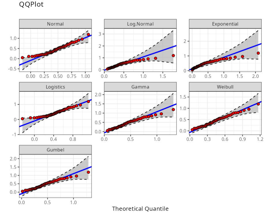
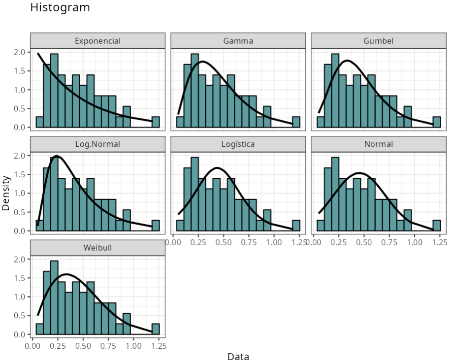
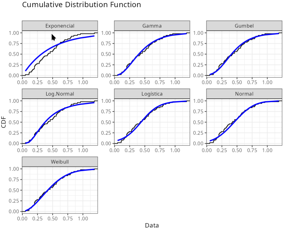
Analysis result

	Graphical analysis