4. Performance Indices - Pp (Discrete Data)
In some applications, we are interested in evaluating the capacity of a process in which we only observe whether the product is within or outside specifications, that is, the data collected is of a discrete nature.
Example 1:
An industry is interested in analyzing the capacity of a process in which the number of non-conforming points on a steel blade is checked, each blade measuring 50 $\text{cm}^2$ . The data is shown in the following table
| Sample | No non conforming | Sample size cm2 |
|---|---|---|
| 1 | 2 | 50 |
| 2 | 4 | 50 |
| 3 | 3 | 50 |
| 4 | 1 | 50 |
| 5 | 2 | 50 |
| 6 | 5 | 50 |
| 7 | 2 | 50 |
| 8 | 5 | 50 |
| 9 | 4 | 50 |
| 10 | 1 | 50 |
| 11 | 6 | 50 |
| 12 | 3 | 50 |
| 13 | 3 | 50 |
| 14 | 6 | 50 |
| 15 | 1 | 50 |
| 16 | 4 | 50 |
| 17 | 1 | 50 |
| 18 | 8 | 50 |
| 19 | 1 | 50 |
| 20 | 4 | 50 |
| 21 | 4 | 50 |
| 22 | 2 | 50 |
| 23 | 4 | 50 |
| 24 | 2 | 50 |
| 25 | 1 | 50 |
| 26 | 2 | 50 |
| 27 | 2 | 50 |
| 28 | 3 | 50 |
| 29 | 4 | 50 |
| 30 | 4 | 50 |
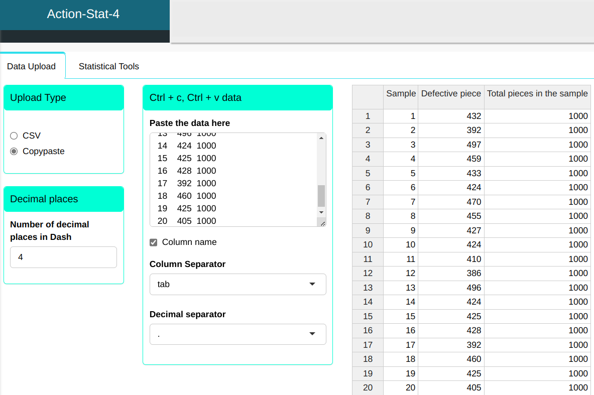
We will upload the data to the system.
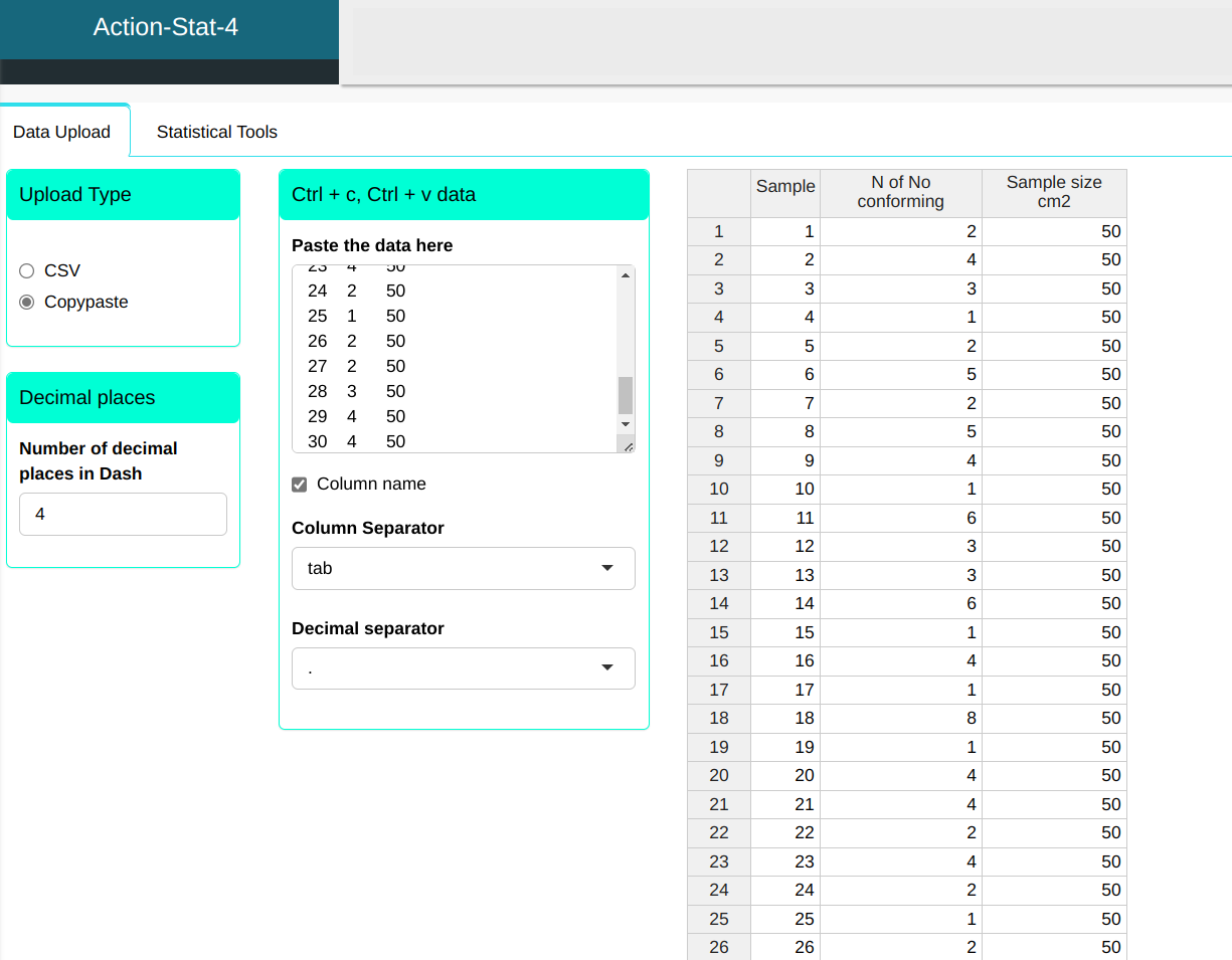
Setting as shown in the figure below to perform the analysis
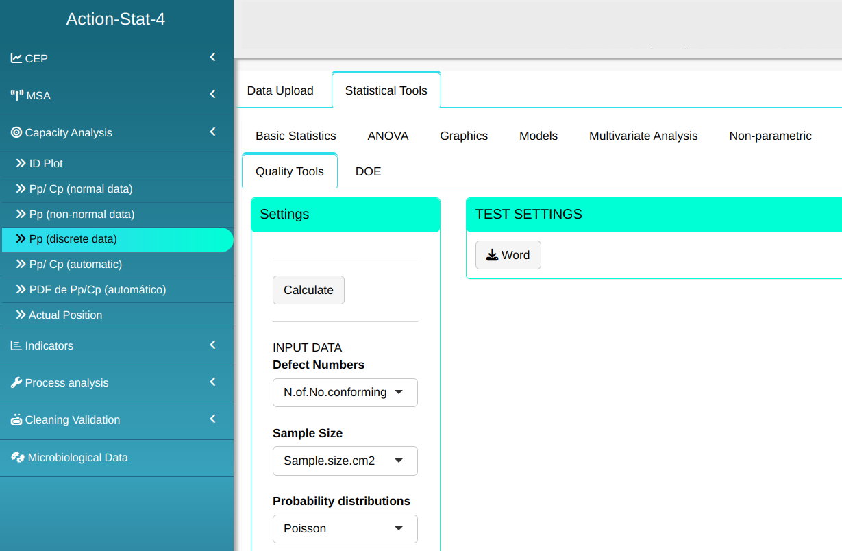

- In “select tests” we can choose the tests we want to carry out.
Then click Calculate we obtain the results. You can also generate the analyses and download them in Word format.

The results are:
Defect mean:
| V1 | |
|---|---|
| Target % (Optional) | 0.000 |
| Defect Mean: | 3.133 |
| Lower Limit: | 2.532 |
| Upper Limit: | 3.834 |
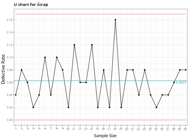
DPU Mean:
| V1 | |
|---|---|
| DPU Mean: | 0.063 |
| Lower Limit: | 0.051 |
| Upper Limit: | 0.077 |
| Minimum: | 0.020 |
| Maximum: | 0.160 |
Confidence Intervals (PPM)
| V1 | |
|---|---|
| PPM’s Mean: | 60743.49 |
| Lower Limit: | 49380.16 |
| Upper Limit: | 73821.34 |
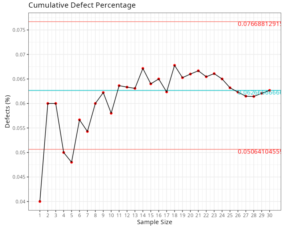
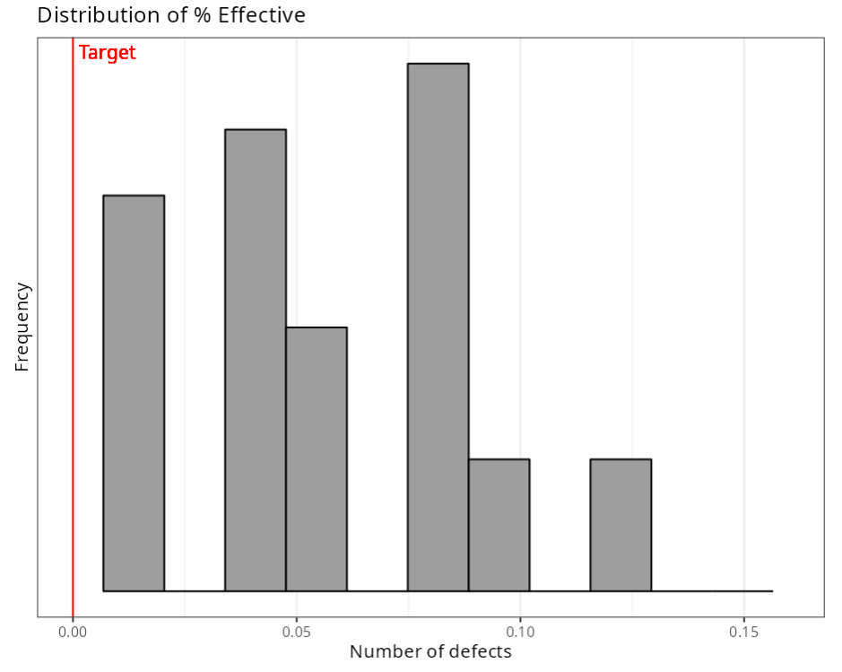
Analysis result
| Defect | Sample size | Percentage of defect | accumulated defect | Accumalated total | Accumulated percentagem |
|---|---|---|---|---|---|
| 2 | 50 | 0.04 | 2 | 50 | 0.04 |
| 4 | 50 | 0.08 | 6 | 100 | 0.06 |
| 3 | 50 | 0.06 | 9 | 150 | 0.06 |
| 1 | 50 | 0.02 | 10 | 200 | 0.05 |
| 2 | 50 | 0.04 | 12 | 250 | 0.048 |
| 5 | 50 | 0.1 | 17 | 300 | 0.057 |
| 2 | 50 | 0.04 | 19 | 350 | 0.054 |
| 5 | 50 | 0.1 | 24 | 400 | 0.06 |
| 4 | 50 | 0.08 | 28 | 450 | 0.062 |
| 1 | 50 | 0.02 | 29 | 500 | 0.058 |
| 6 | 50 | 0.12 | 35 | 550 | 0.064 |
| 3 | 50 | 0.06 | 38 | 600 | 0.063 |
| 3 | 50 | 0.06 | 41 | 650 | 0.063 |
| 6 | 50 | 0.12 | 47 | 700 | 0.067 |
| 1 | 50 | 0.02 | 48 | 750 | 0.064 |
| 4 | 50 | 0.08 | 52 | 800 | 0.065 |
| 1 | 50 | 0.02 | 53 | 850 | 0.062 |
| 8 | 50 | 0.16 | 61 | 900 | 0.068 |
| 1 | 50 | 0.02 | 62 | 950 | 0.065 |
| 4 | 50 | 0.08 | 66 | 1.000 | 0.066 |
| 4 | 50 | 0.08 | 70 | 1.050 | 0.067 |
| 2 | 50 | 0.04 | 72 | 1.100 | 0.065 |
| 4 | 50 | 0.08 | 76 | 1.150 | 0.066 |
| 2 | 50 | 0.04 | 78 | 1.200 | 0.065 |
| 1 | 50 | 0.02 | 79 | 1.250 | 0.063 |
| 2 | 50 | 0.04 | 81 | 1.300 | 0.062 |
| 2 | 50 | 0.04 | 83 | 1.350 | 0.061 |
| 3 | 50 | 0.06 | 86 | 1.400 | 0.061 |
| 4 | 50 | 0.08 | 90 | 1.450 | 0.062 |
| 4 | 50 | 0.08 | 94 | 1.500 | 0.063 |
Example 2:
An industry is interested in analyzing the capacity of a pieces process in which the proportion of defective in lots of 1000 pieces is checked. The data is shown in the table below.
| Sample | Defective pieces | Total pieces in the sample |
|---|---|---|
| 1 | 432 | 1000 |
| 2 | 392 | 1000 |
| 3 | 497 | 1000 |
| 4 | 459 | 1000 |
| 5 | 433 | 1000 |
| 6 | 424 | 1000 |
| 7 | 470 | 1000 |
| 8 | 455 | 1000 |
| 9 | 427 | 1000 |
| 10 | 424 | 1000 |
| 11 | 410 | 1000 |
| 12 | 386 | 1000 |
| 13 | 496 | 1000 |
| 14 | 424 | 1000 |
| 15 | 425 | 1000 |
| 16 | 428 | 1000 |
| 17 | 392 | 1000 |
| 18 | 460 | 1000 |
| 19 | 425 | 1000 |
| 20 | 405 | 1000 |
We will upload the data to the system.
Setting as shown in the figure below to perform the analysis
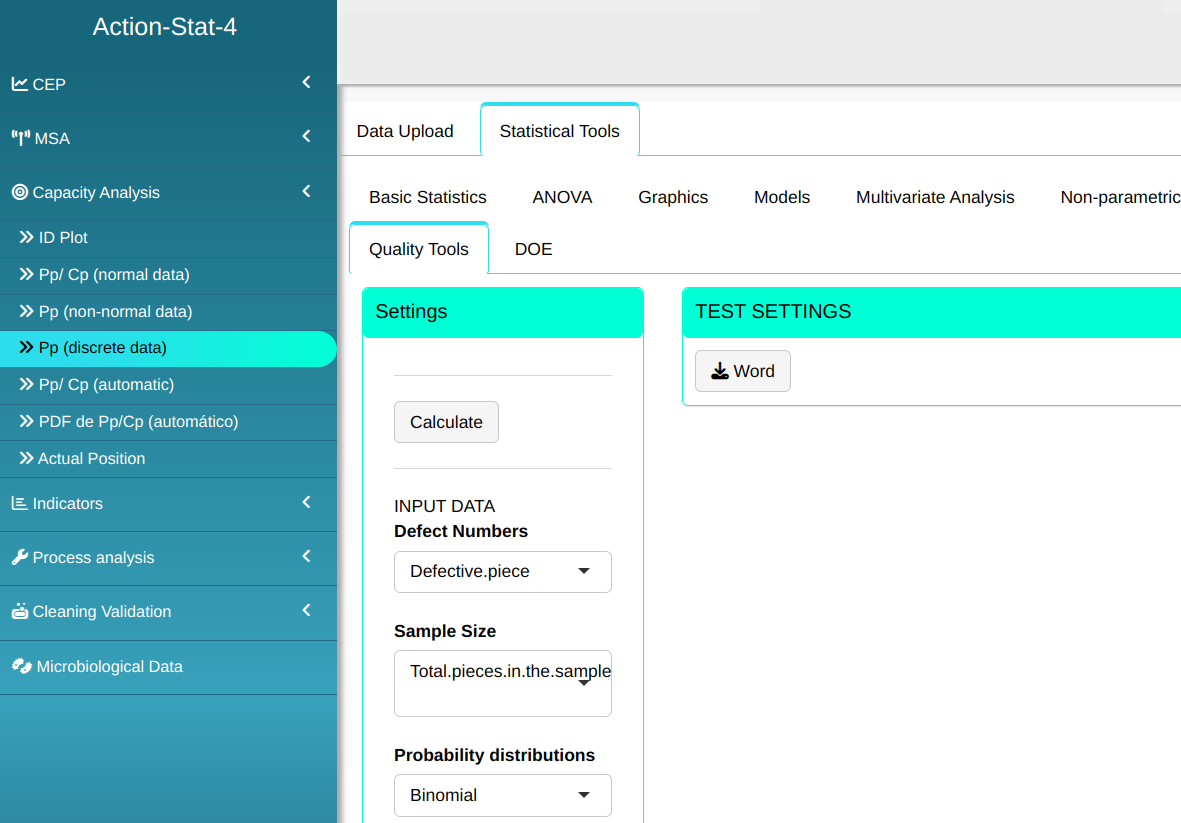

- In “select tests” we can choose the tests we want to carry out.
Then click Calculate we obtain the results. You can also generate the analyses and download them in Word format.
The results are
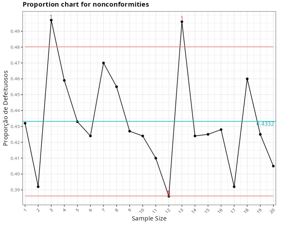
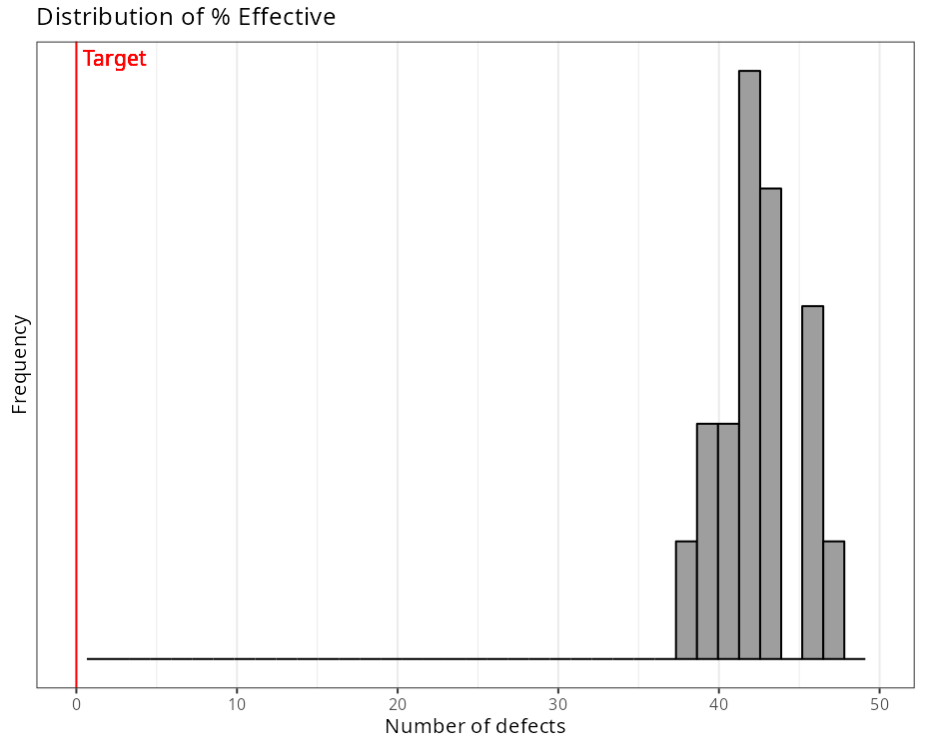
Defect percentage:
| V1 | |
|---|---|
| Target % (Optional) | 0.000 |
| Defect percentage: | 43.320 |
| Lower Limit: | 42.632 |
| Upper Limit: | 44.010 |
Defect Rate:
| V1 | |
|---|---|
| Defect rate: | 0.4332 |
| Lower Limit: | 0.4263 |
| Upper Limit: | 0.4401 |
ICP
| V1 | |
|---|---|
| ICP | 0.168 |
| Lower Limit: | 0.186 |
| Upper Limit: | 0.151 |
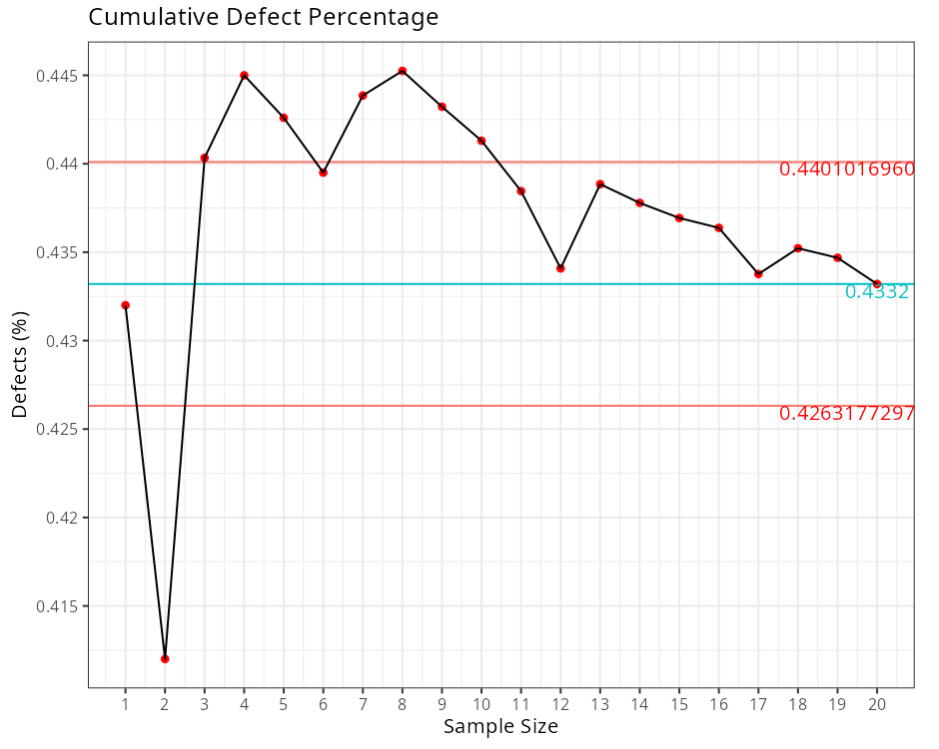
Results analysis
| Defect | Sample size | percentage of defect | Accumulated defect | Accumulated total | Accumulated percentage |
|---|---|---|---|---|---|
| 432 | 1000 | 0.432 | 432 | 1000 | 0.432 |
| 392 | 1000 | 0.392 | 824 | 2000 | 0.412 |
| 497 | 1000 | 0.497 | 1321 | 3000 | 0.44 |
| 459 | 1000 | 0.459 | 1780 | 4000 | 0.445 |
| 433 | 1000 | 0.433 | 2213 | 5000 | 0.443 |
| 424 | 1000 | 0.424 | 2637 | 6000 | 0.44 |
| 470 | 1000 | 0.47 | 3107 | 7000 | 0.444 |
| 455 | 1000 | 0.455 | 3562 | 8000 | 0.445 |
| 427 | 1000 | 0.427 | 3989 | 9000 | 0.443 |
| 424 | 1000 | 0.424 | 4413 | 10000 | 0.441 |
| 410 | 1000 | 0.41 | 4823 | 11000 | 0.438 |
| 386 | 1000 | 0.386 | 5209 | 12000 | 0.434 |
| 496 | 1000 | 0.496 | 5705 | 13000 | 0.439 |
| 424 | 1000 | 0.424 | 6129 | 14000 | 0.438 |
| 425 | 1000 | 0.425 | 6554 | 15000 | 0.437 |
| 428 | 1000 | 0.428 | 6982 | 16000 | 0.436 |
| 392 | 1000 | 0.392 | 7374 | 17000 | 0.434 |
| 460 | 1000 | 0.46 | 7834 | 18000 | 0.435 |
| 425 | 1000 | 0.425 | 8259 | 19000 | 0.435 |
| 405 | 1000 | 0.405 | 8664 | 20000 | 0.433 |