3. Performance Indices - Pp (Non-normal Data)
In many situations we are interested in evaluating the performance of a production process on a given characteristic. However, the normal distribution may not fit the data well. In this situation, we can find an alternative probability distribution or use a non-parametric method.
Example 1:
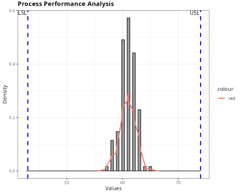
Let’s consider the data in the table below referring to measurements of the diameter of a cylinder number 3, taken suddenly and taking 5 pieces every 20 produced. The specifications for this data are: USL = 74 and LSL = 43.
| Date | Hour | Sheets | M1 | M2 | M3 | M4 | M5 |
|---|---|---|---|---|---|---|---|
| 26/abr | 11:40 | 14650 | 61 | 62 | 60 | 61 | 60 |
| 26/abr | 13:10 | 14650 | 62 | 61 | 62 | 63 | 62 |
| 26/abr | 17:15 | 19730 | 61 | 58 | 61 | 60 | 60 |
| 26/abr | 21:35 | 19730 | 62 | 60 | 62 | 61 | 60 |
| 28/abr | 7:08 | 14650 | 63 | 62 | 61 | 60 | 62 |
| 28/abr | 8:15 | 14650 | 62 | 61 | 58 | 59 | 60 |
| 28/abr | 10:03 | 14650 | 62 | 61 | 60 | 62 | 61 |
| 28/abr | 12:44 | 14650 | 62 | 61 | 60 | 58 | 59 |
| 28/abr | 14:12 | 14650 | 62 | 61 | 60 | 60 | 61 |
| 28/abr | 17:20 | 19730 | 61 | 60 | 60 | 61 | 63 |
| 28/abr | 19:20 | 19730 | 59 | 61 | 60 | 59 | 61 |
| 28/abr | 22:30 | 19730 | 61 | 60 | 62 | 62 | 60 |
| 29/abr | 7:28 | 14650 | 62 | 61 | 60 | 58 | 57 |
| 29/abr | 8:40 | 14650 | 61 | 60 | 59 | 58 | 58 |
| 29/abr | 11:36 | 14650 | 62 | 61 | 60 | 61 | 61 |
| 29/abr | 12:50 | 14650 | 61 | 60 | 62 | 61 | 62 |
| 29/abr | 14:18 | 14650 | 62 | 61 | 63 | 62 | 63 |
| 29/abr | 18:15 | 19730 | 61 | 63 | 63 | 62 | 61 |
| 29/abr | 22:45 | 19730 | 60 | 59 | 60 | 61 | 60 |
| 30/abr | 10:01 | 14650 | 63 | 62 | 61 | 60 | 62 |
| 30/abr | 12:20 | 14650 | 61 | 60 | 59 | 58 | 59 |
| 30/abr | 16:50 | 19730 | 63 | 61 | 63 | 62 | 61 |
| 30/abr | 18:15 | 19730 | 61 | 60 | 60 | 59 | 60 |
| 30/abr | 21:35 | 19730 | 63 | 65 | 63 | 64 | 63 |
| 5/mai | 12:58 | 14650 | 61 | 62 | 63 | 62 | 60 |
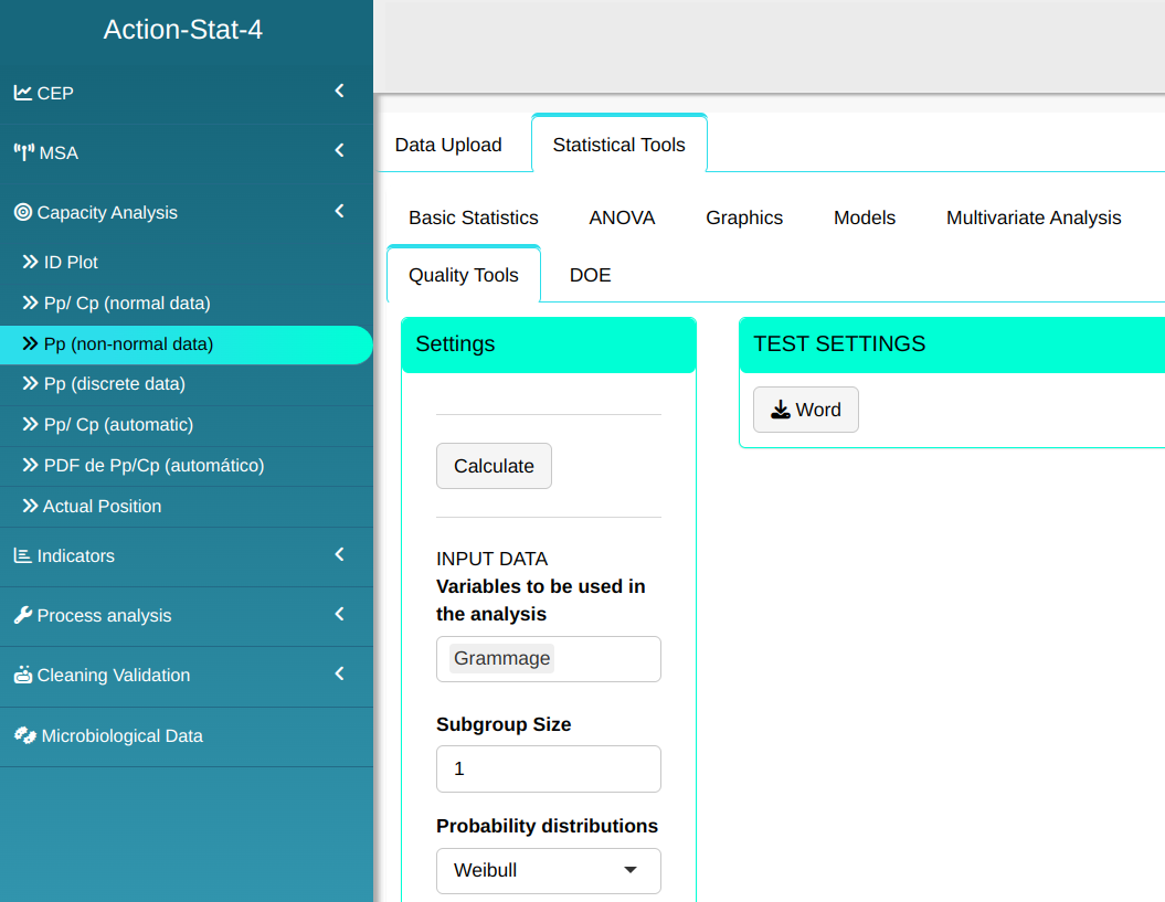
We will upload the data to the system.
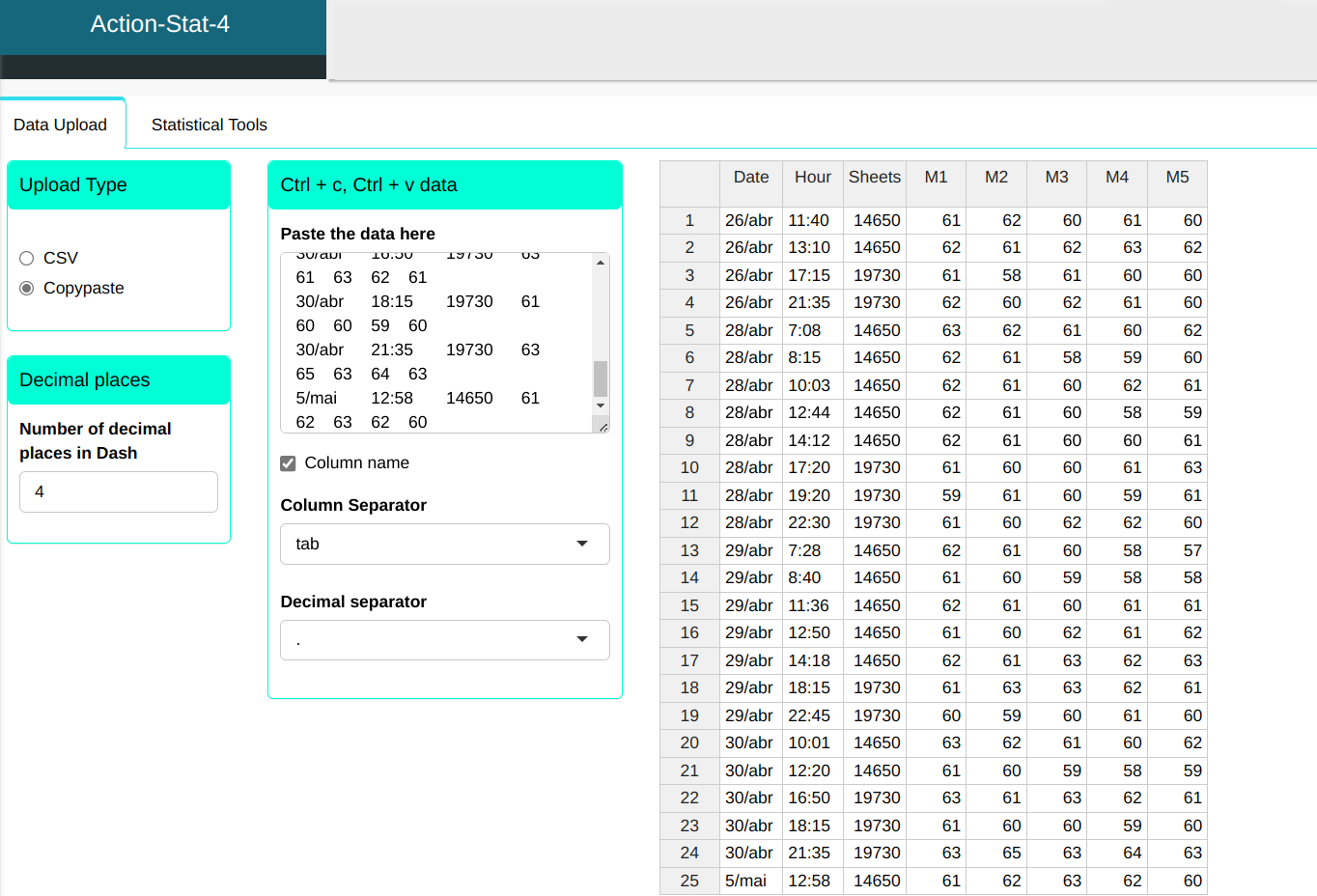
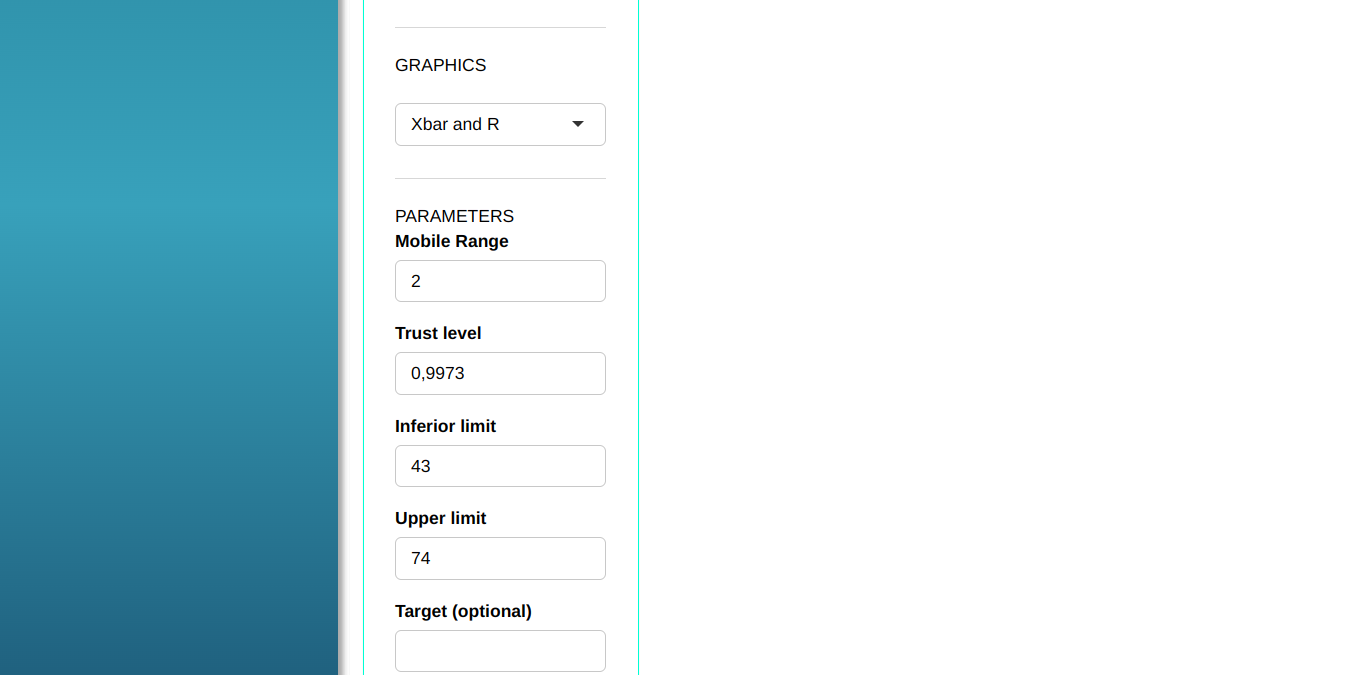
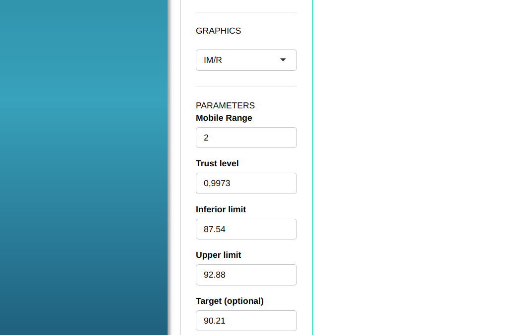
Setting as shown in the figure below to perform the analysis
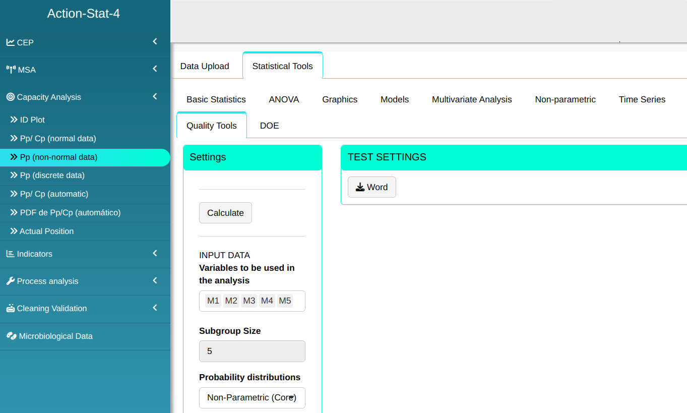

- In “Select Tests” we can choose the tests we want to perform.
Then click Calculate we obtain the results. You can also generate the analyses and download them in Word format.

The results are
Specifications
| Value | |
|---|---|
| Sample: | 125 |
| Lower Limit | 43 |
| Upper Limit | 74 |
Estimates
| Parameters | Value |
|---|---|
| Average: | 60.912 |
| Standard Deviation: | 1.42566339962568 |
PERFORMANCE INDICES
| Performance Indices | |
|---|---|
| PP | 3.4431 |
| PPL | 4.0347 |
| PPU | 2.8655 |
| PPk | 2.8655 |
Observed Indices
| Observed Indices | |
|---|---|
| PPM > LSE | 0 |
| PPM < LIE | 0 |
| PPM Total | 0 |
Expected rates
| Expected rates | |
|---|---|
| PPM > USL | 0 |
| PPM < LSL | 0 |
| PPM Total | 0 |
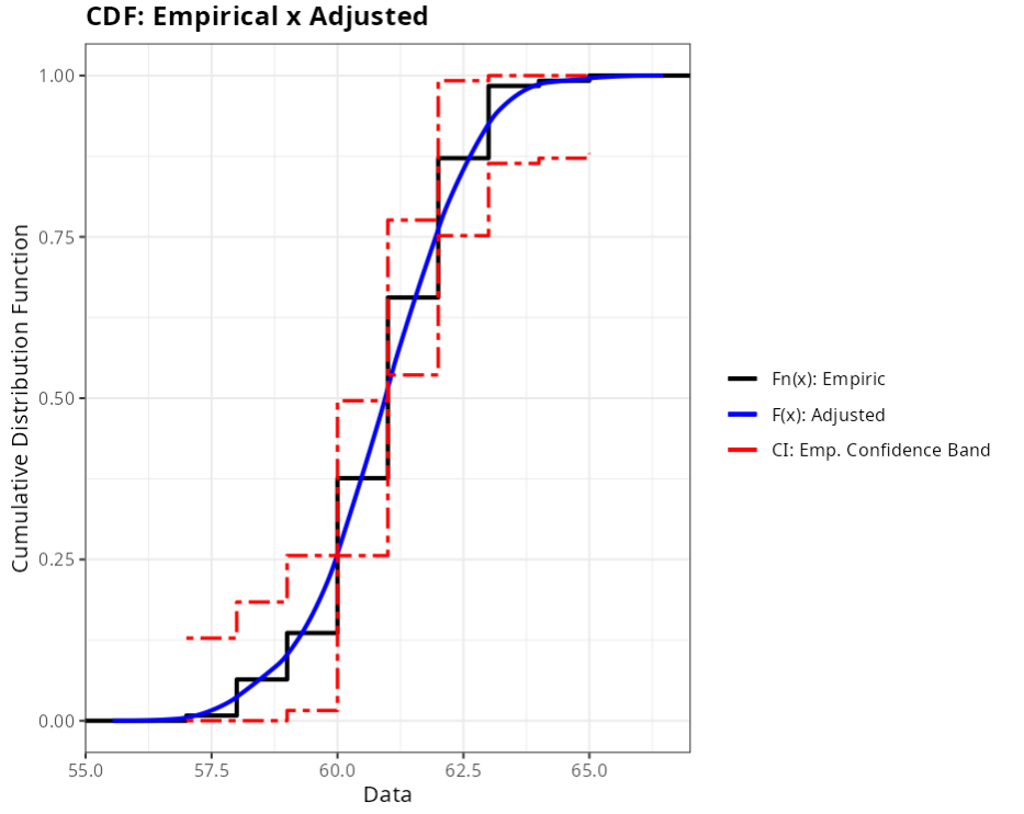
Adjustment Quality (No Parametric (Kernel): Method triangular)
| Method | Statistics | P-value | |
|---|---|---|---|
| Cramér-von Mises | triangular | 1.089 | 0.219 |
| Kolmogorov-Smirnov | triangular | 0.144 | 0.150 |
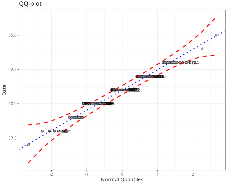
Normality test (Outliers)
| Obs. | Normal Quantiles | Data | Criterion |
|---|---|---|---|
| 19 | -1.08 | 60 | Envelope (Confidence Level = 95%) |
| 29 | -1.05 | 60 | Envelope (Confidence Level=95%) |
| 35 | -1.01 | 60 | Envelope (Confidence Level=95%) |
| 37 | -0.98 | 60 | Envelope (Confidence Level=95%) |
| 39 | -0.95 | 60 | Envelope (Confidence Level=95%) |
| 1 | -0.31 | 61 | Envelope (Confidence Level=95%) |
| 3 | -0.28 | 61 | Envelope (Confidence Level=95%) |
| 10 | -0.26 | 61 | Envelope (Confidence Level=95%) |
| 12 | -0.24 | 61 | Envelope (Confidence Level=95%) |
| 14 | -0.22 | 61 | Envelope (Confidence Level=95%) |
| 2 | 0.41 | 62 | Envelope (Confidence Level=95%) |
| 4 | 0.43 | 62 | Envelope (Confidence Level=95%) |
| 96 | -1.63 | 58 | Envelope (Confidence Level=95%) |
| 114 | -1.55 | 58 | Envelope (Confidence Level=95%) |
| 104 | -0.43 | 60 | Envelope (Confidence Level=95%) |
| 106 | -0.41 | 60 | Envelope (Confidence Level=95%) |
| 112 | -0.39 | 60 | Envelope (Confidence Level=95%) |
| 119 | -0.37 | 60 | Envelope (Confidence Level=95%) |
| 123 | -0.35 | 60 | Envelope (Confidence Level=95%) |
| 125 | -0.33 | 60 | Envelope (Confidence Level=95%) |
| 90 | 0.22 | 61 | Envelope (Confidence Level=95%) |
| 91 | 0.24 | 61 | Envelope (Confidence Level=95%) |
| 94 | 0.26 | 61 | Envelope (Confidence Level=95%) |
| 107 | 0.28 | 61 | Envelope (Confidence Level=95%) |
| 109 | 0.31 | 61 | Envelope (Confidence Level=95%) |
| 111 | 0.33 | 61 | Envelope (Confidence Level=95%) |
| 115 | 0.35 | 61 | Envelope (Confidence Level=95%) |
| 118 | 0.37 | 61 | Envelope (Confidence Level=95%) |
| 122 | 0.39 | 61 | Envelope (Confidence Level=95%) |
| 97 | 0.95 | 62 | Envelope (Confidence Level=95%) |
| 100 | 0.98 | 62 | Envelope (Confidence Level=95%) |
| 102 | 1.01 | 62 | Envelope (Confidence Level=95%) |
| 105 | 1.05 | 62 | Envelope (Confidence Level=95%) |
| 116 | 1.08 | 62 | Envelope (Confidence Level=95%) |
| 120 | 1.12 | 62 | Envelope (Confidence Level=95%) |
| 110 | 1.8 | 63 | Envelope (Confidence Level=95%) |
| 117 | 1.91 | 63 | Envelope (Confidence Level=95%) |
| 124 | 2.05 | 63 | Envelope (Confidence Level=95%) |
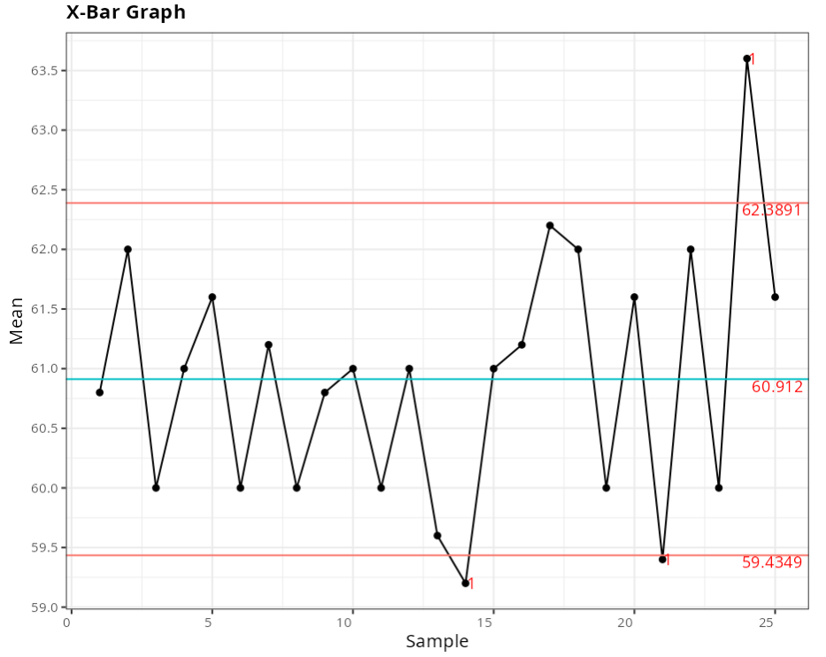
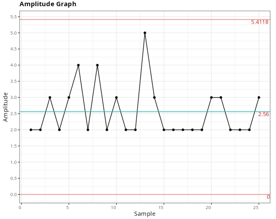
Out-of-control points - X-Barra Graph
| Subgroup | Value | Test |
|---|---|---|
| 14 | 59.2 | 1 point greater than 3 sigmas from the center line |
| 21 | 59.4 | 1 point greater than 3 sigmas from the center line |
| 24 | 63.6 | 1 point greater than 3 sigmas from the center line |
Example 2:
The data used in this example refers to the grammage (gr/m^2^) of a sheet of paper. The specifications for this data are USL = 92.88; Target = 90.21 and LSL = 87.54.
| Grammage gr/m2 |
|---|
| 88.20 |
| 88.90 |
| 90.50 |
| 90.30 |
| 90.00 |
| 90.20 |
| 91.20 |
| 91.00 |
| 91.50 |
| 91.40 |
| 91.30 |
| 90.20 |
| 91.40 |
| 89.90 |
| 90.20 |
| 90.10 |
| 90.80 |
| 91.40 |
| 91.30 |
| 89.00 |
| 90.70 |
| 89.50 |
| 91.20 |
| 90.50 |
| 90.60 |
We will upload the data to the system.
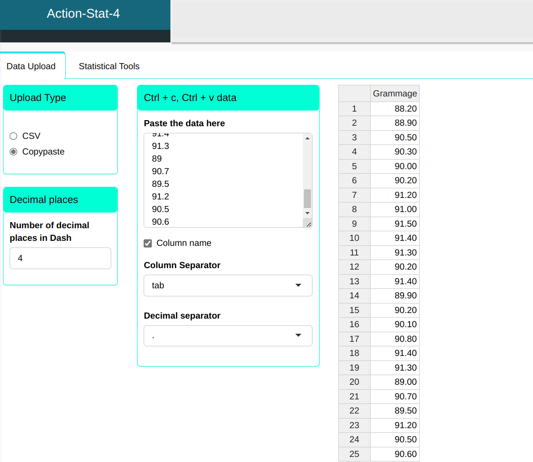
Setting as shown in the figure below to perform the analysis

- In “select tests” we can choose the tests we want to carry out.
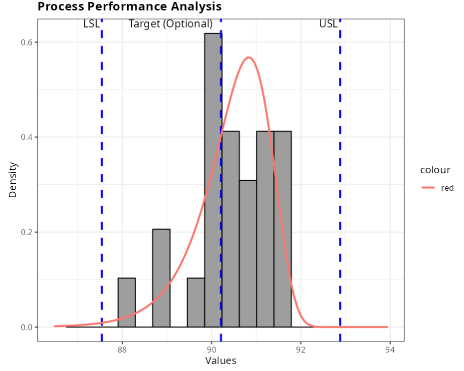
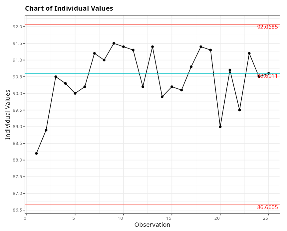
Then click Calculate we obtain the results. You can also generate the analyses and download them in Word format.
The results are
Specifications
| Value | |
|---|---|
| Sample: | 25 |
| Lower Limit | 87.54 |
| Target (Optional) | 90.21 |
| Upper Limit | 92.88 |
Estimates
| Parameters | Value |
|---|---|
| Average: | 90.4689587801872 |
| Standard Deviation: | 0.822555917720036 |
| Forma: | 140.336103078599 |
| Scale: | 90.8380519338829 |
Performance Indices
| Performance Indices | |
|---|---|
| PP | 0.987 |
| PPL | 0.777 |
| PPU | 1.553 |
| PPk | 0.777 |
Observed Indices
| Observed Indices | |
|---|---|
| PPM > USL | 0 |
| PPM < USL | 0 |
| PPM Total | 0 |
Expected Indices
| Expected Indices | |
|---|---|
| PPM > USL | 0.000147211465240105 |
| PPM < LSL | 5556.66966289269 |
| PPM Total | 5556.66981010415 |
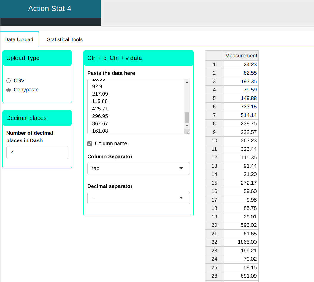
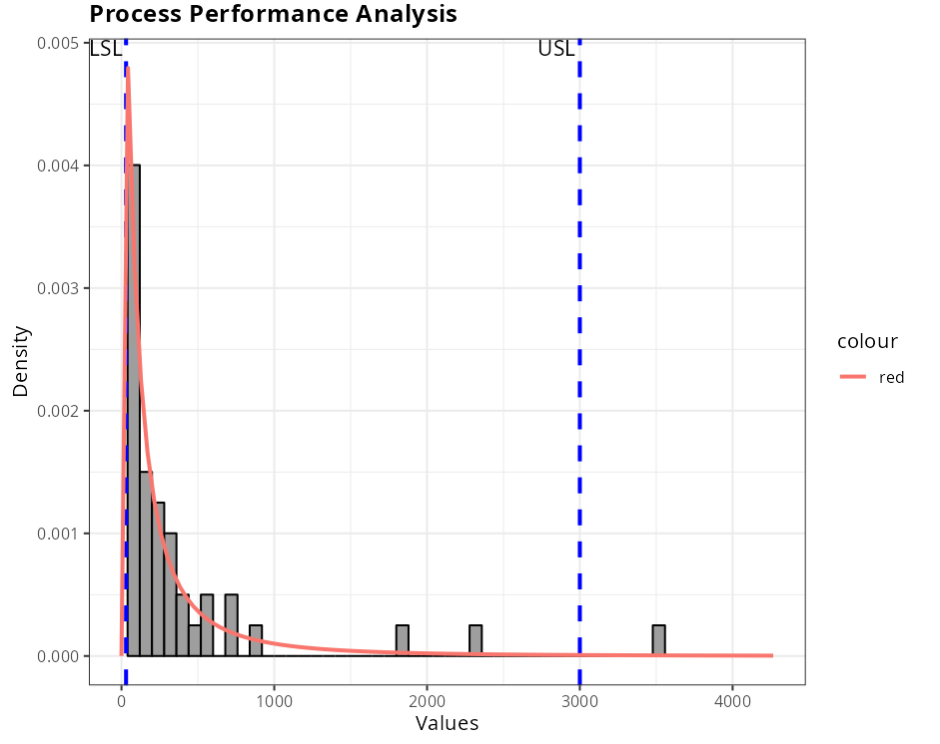
Example 3:
Let’s consider the measurement data in the table below. The specifications for this data are USL = 3000 and LSL = 30.
| Measurement |
|---|
| 24.23 |
| 62.55 |
| 193.35 |
| 79.59 |
| 149.88 |
| 733.15 |
| 514.14 |
| 238.75 |
| 222.57 |
| 363.23 |
| 323.44 |
| 115.35 |
| 91.44 |
| 31.2 |
| 272.17 |
| 59.6 |
| 9.98 |
| 85.78 |
| 29.01 |
| 593.02 |
| 61.65 |
| 1865 |
| 199.21 |
| 79.02 |
| 58.15 |
| 691.09 |
| 42.43 |
| 51.42 |
| 342.19 |
| 138.81 |
| 8.61 |
| 127.5 |
| 309.33 |
| 17.11 |
| 2300.26 |
| 244.52 |
| 7.68 |
| 83.97 |
| 45.33 |
| 520.4 |
| 3556.16 |
| 59.75 |
| 10.53 |
| 92.9 |
| 217.09 |
| 115.66 |
| 425.71 |
| 296.95 |
| 867.67 |
| 161.08 |
We will upload the data to the system.
Setting as shown in the figure below to perform the analysis
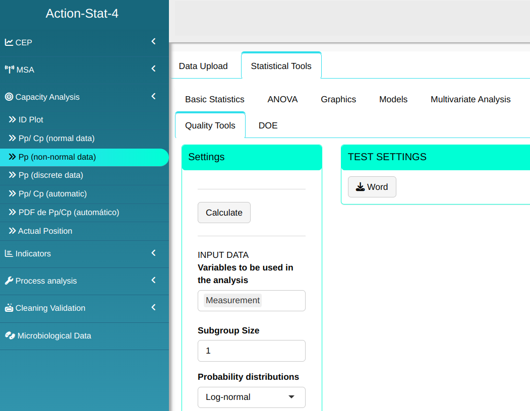
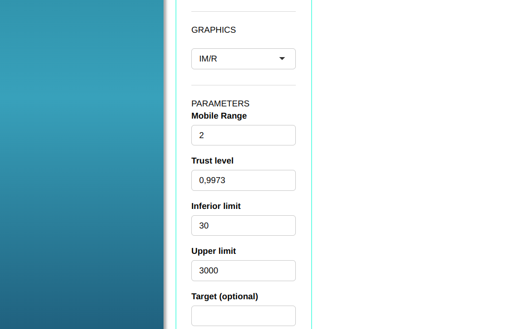

- In “select tests” we can choose the tests we want to carry out.
Then click Calculate we obtain the results. You can also generate the analyses and download them in Word format.
The results are
Specifications
| Value | |
|---|---|
| Sample: | 50 |
| Lower Limit | 30 |
| Upper Limit | 3000 |
Estimates
| Parameters | Value |
|---|---|
| Average: | 358.584811836873 |
| Standard Deviation: | 890.343884308414 |
Performance Indices
| Performance Indices | |
|---|---|
| PP | 0.329 |
| PPL | 0.788 |
| PPU | 0.322 |
| PPk | 0.322 |
Observed Indices
| Observed Indices | |
|---|---|
| PPM > USL | 20000 |
| PPM < LSL | 140000 |
| PPM Total | 160000 |
Expected Indices
| Expected Indices | |
|---|---|
| PPM > USL | 13367.0406498871 |
| PPM < LSL | 143137.013200317 |
| PPM Total | 156504.053850204 |
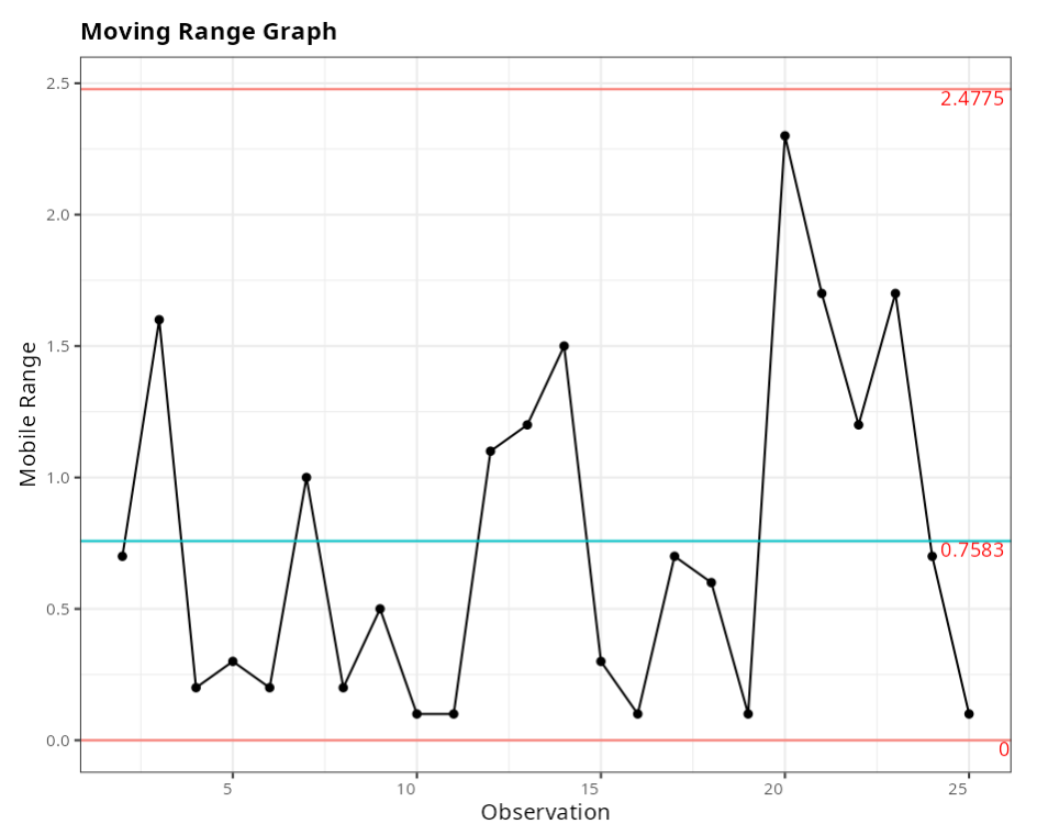
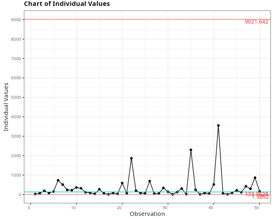
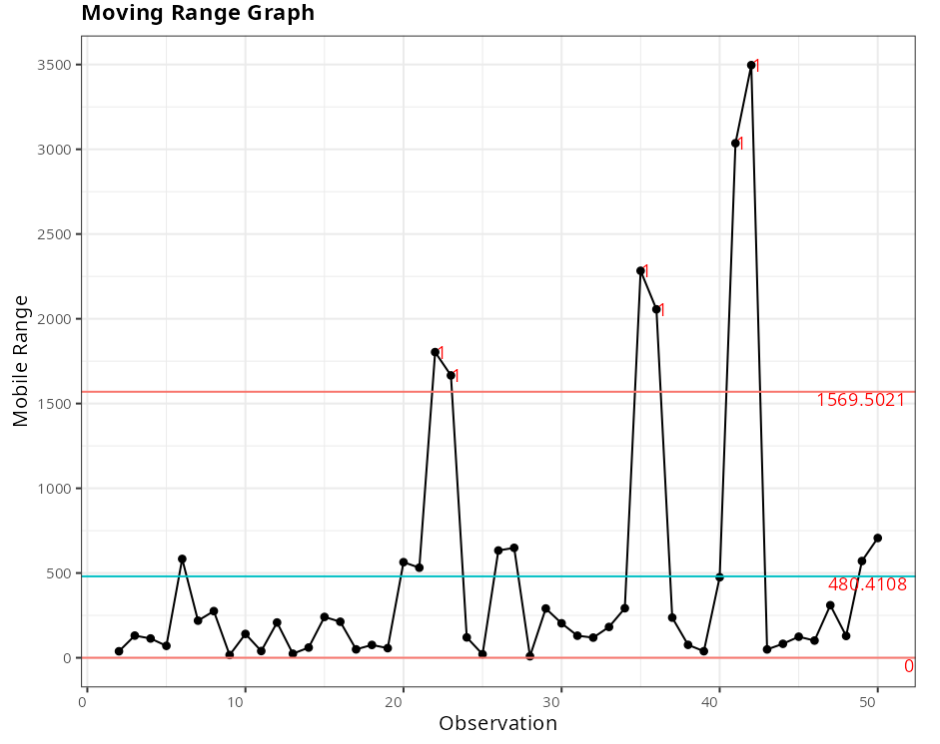
Out-of-control points - Moving Range Graph
| Subgroup | Value | Test |
|---|---|---|
| 22 | 1803.35 | 1 point greater than 3 Sigmas from the center line |
| 23 | 1665.79 | 1 point greater than 3 Sigmas from the center line |
| 35 | 2283.15 | 1 point greater than 3 Sigmas from the center line |
| 36 | 2055.74 | 1 point greater than 3 Sigmas from the center line |
| 41 | 3035.76 | 1 point greater than 3 Sigmas from the center line |
| 42 | 3496.41 | 1 point greater than 3 Sigmas from the center line |
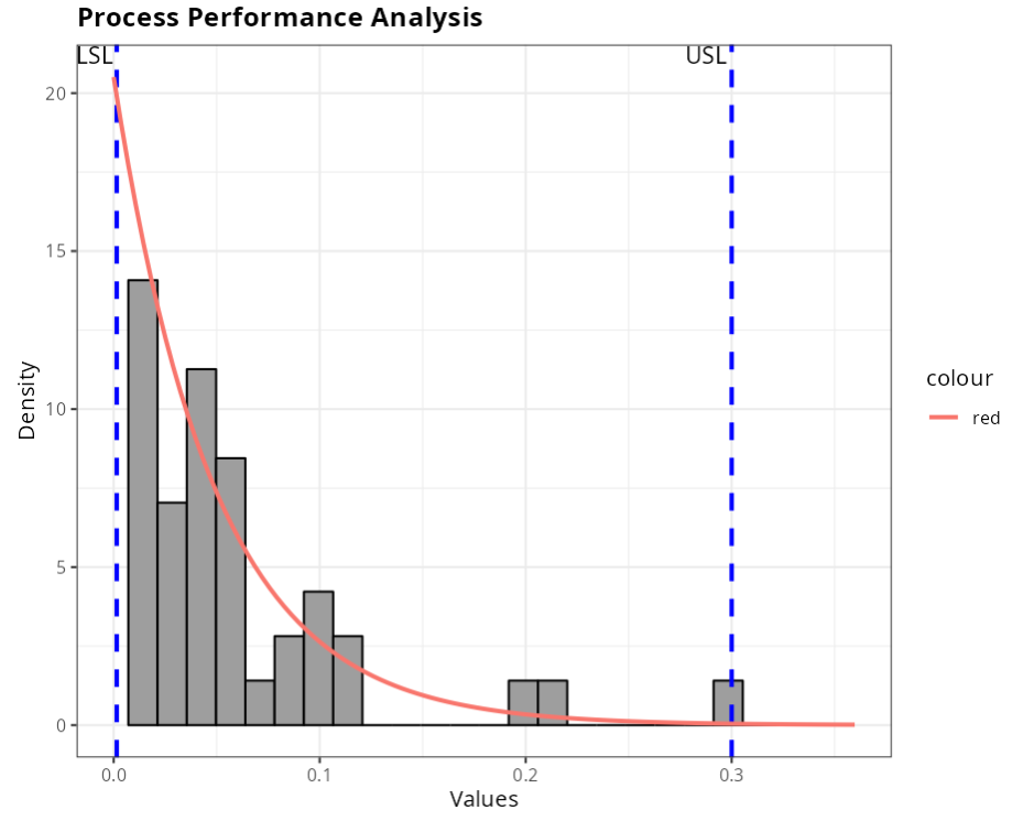
Example 4:
Let’s consider the data in the table below relating to measurements of a particular piece. The specifications for this data are USEL = 0.3 and LSL = 0.0015.
| Measurements |
|---|
| 0.106 |
| 0.007 |
| 0.007 |
| 0.014 |
| 0.052 |
| 0.058 |
| 0.003 |
| 0.03 |
| 0.03 |
| 0.041 |
| 0.012 |
| 0.015 |
| 0.011 |
| 0.002 |
| 0.02 |
| 0.292 |
| 0.059 |
| 0.04 |
| 0.016 |
| 0.023 |
| 0.039 |
| 0.036 |
| 0.087 |
| 0.075 |
| 0.008 |
| 0.04 |
| 0.206 |
| 0.002 |
| 0.114 |
| 0.052 |
| 0.009 |
| 0.007 |
| 0.049 |
| 0.094 |
| 0.003 |
| 0.036 |
| 0.101 |
| 0.047 |
| 0.002 |
| 0.114 |
| 0.023 |
| 0.017 |
| 0.03 |
| 0.201 |
| 0.011 |
| 0.055 |
| 0.055 |
| 0.08 |
| 0.002 |
| 0.005 |
We will upload the data to the system.
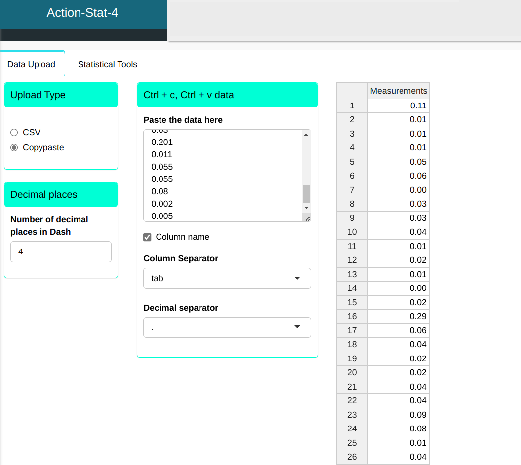
Setting as shown in the figure below to perform the analysis
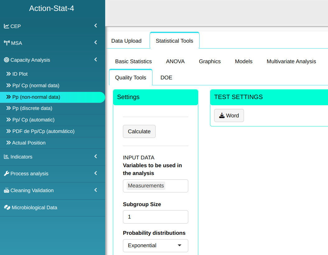
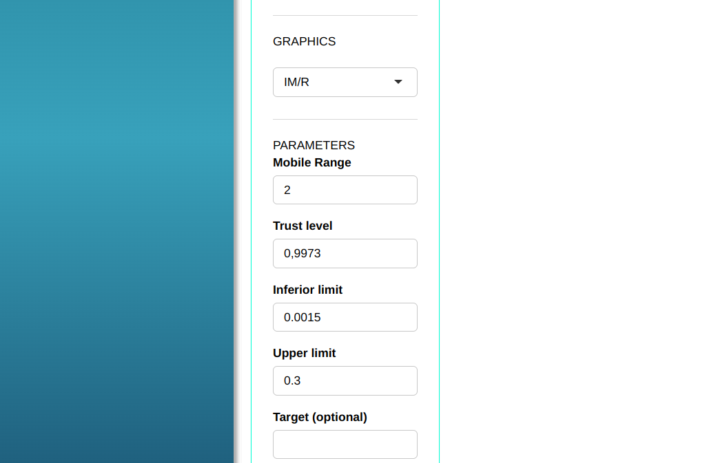

- In “select tests” we can choose the tests we want to carry out.
Then click Calculate we obtain the results. You can also generate the analyses and download them in Word format.
The results are
Specifications
| Value | |
|---|---|
| Sample: | 50 |
| Lower Limit | 0.0015 |
| Upper Limit | 0.3 |
Estimates
| Parameters | Value |
|---|---|
| Average: | 20.5086136177194 |
| Standard Deviation: | 20.5086136177194 |
PERFORMANCE INDICES
| Performance Indices | |
|---|---|
| PP | 0.927 |
| PPL | 0.957 |
| PPU | 0.923 |
| PPk | 0.923 |
Observed Indices
| Observed Indices | |
|---|---|
| PPM > USL | 0 |
| PPM < LSL | 0 |
| PPM Total | 0 |
Expected Indices
| Expected Indices | |
|---|---|
| PPM > USL | 2127.97578815149 |
| PPM < LSL | 30294.556820991 |
| PPM Total | 32422.5326091425 |
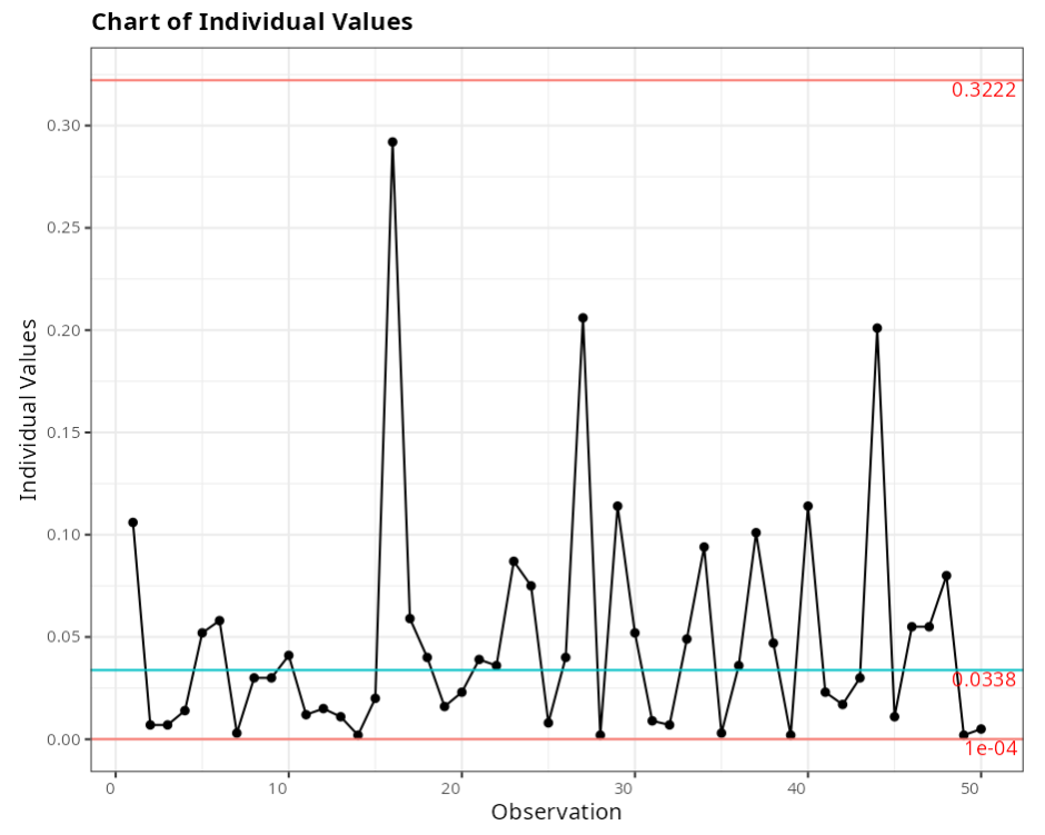
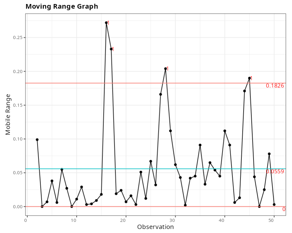
Out-of-control points - Moving Range Graph
| Subgroup | Value | Test |
|---|---|---|
| 16 | 0.272 | 1 point greater than 3 Sigmas from the center line |
| 17 | 0.233 | 1 point greater than 3 Sigmas from the center line |
| 28 | 0.204 | 1 point greater than 3 Sigmas from the center line |
| 45 | 0.190 | 1 point greater than 3 Sigmas from the center line |