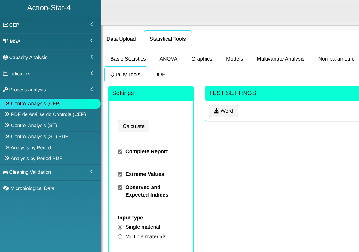
1. Process Analysis (CEP)
ANVISA guidance requires the various pharmaceutical industries to carry out a statistical evaluation of the results of in-process and finished product control. The methodology presented here is well-founded and follows the requirements of the ANVISA Guide (2012). Action Stat provides a statistical tool that allows the generation of complete product quality analysis reports, containing a statistical methodology that follows the following flow: first, an exploratory analysis of the results is carried out with a descriptive summary and a BoxPlot graph. This is followed by a distribution fit test. Next, the stability of the process is assessed using control charts. This is followed by an assessment of the capacity and performance of the process and, finally, a multiple lots comparison test.
Analysis of CEP
To assess the stability of results over time, analysis using CEP graphs is most often used. However, this technique is only recommended in cases where there are not many subgroups of data. The recommendation is a maximum of 150 subgroups to allow proper interpretation of the control chart. In cases where there are more than 150 subgroups, it would be best to perform time series analysis.
Example 1:
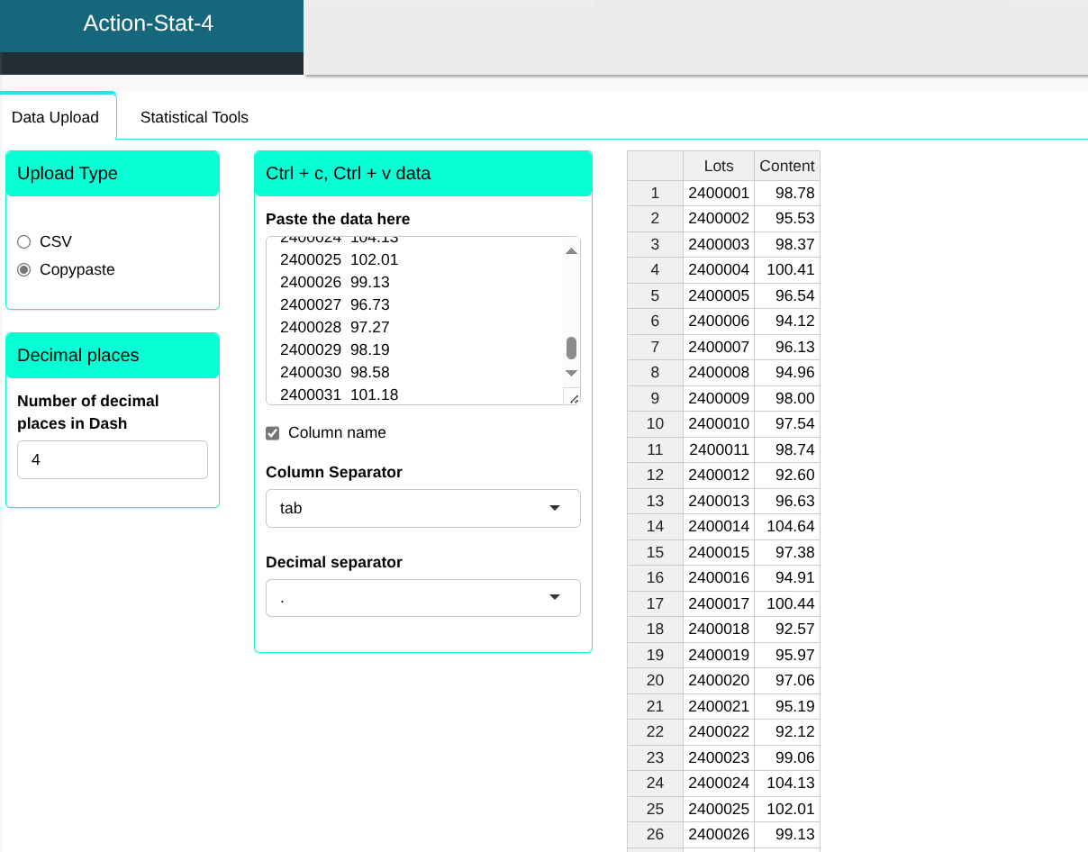
An analyst has measured the content of a substance for 31 production batches of a particular tablet over the course of the year. The aim is to generate a complete statistical report of the process review:
| Lots | Content |
|---|---|
| 2400001 | 98.78 |
| 2400002 | 95.53 |
| 2400003 | 98.37 |
| 2400004 | 100.41 |
| 2400005 | 96.54 |
| 2400006 | 94.12 |
| 2400007 | 96.13 |
| 2400008 | 94.96 |
| 2400009 | 98.00 |
| 2400010 | 97.54 |
| 2400011 | 98.74 |
| 2400012 | 92.60 |
| 2400013 | 96.63 |
| 2400014 | 104.64 |
| 2400015 | 97.38 |
| 2400016 | 94.91 |
| 2400017 | 100.44 |
| 2400018 | 92.57 |
| 2400019 | 95.97 |
| 2400020 | 97.06 |
| 2400021 | 95.19 |
| 2400022 | 92.12 |
| 2400023 | 99.06 |
| 2400024 | 104.13 |
| 2400025 | 102.01 |
| 2400026 | 99.13 |
| 2400027 | 96.73 |
| 2400028 | 97.27 |
| 2400029 | 98.19 |
| 2400030 | 98.58 |
| 2400031 | 101.18 |
We will upload the data to the system.
Configuring as shown in the figure below to perform the analysis.
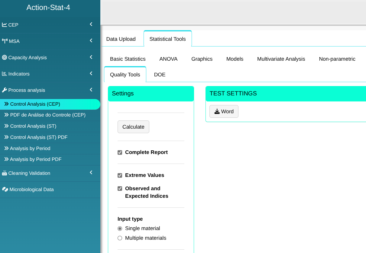
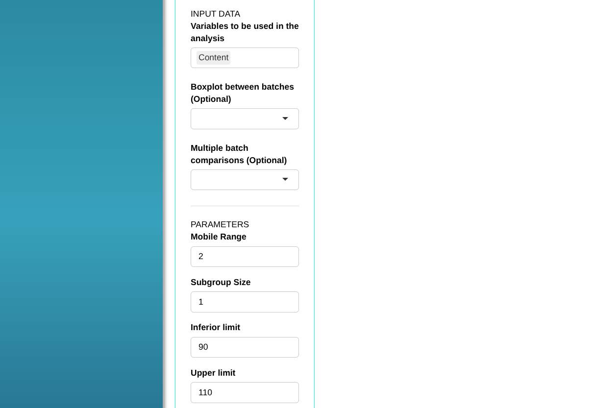
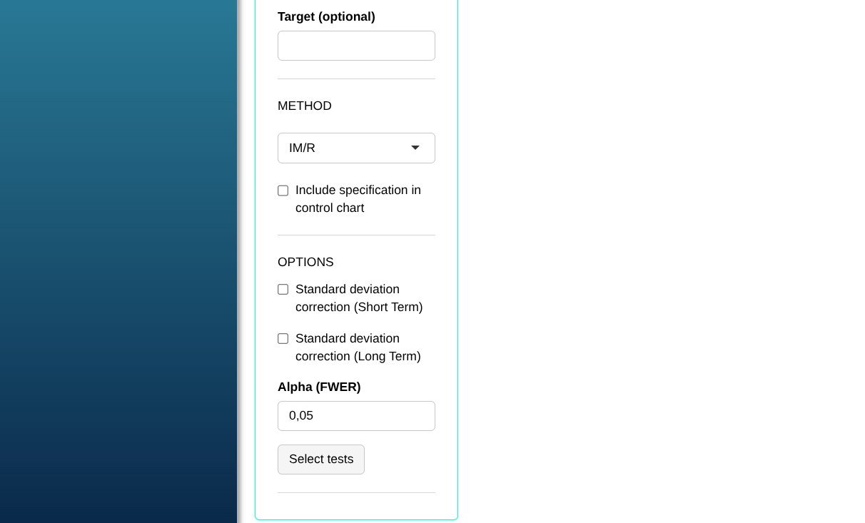
Then click Calculate we obtain the results. You can also generate the analyses and download them in Word format.
Los resultados son:
Descriptive summary
| Statistics | |
|---|---|
| Minimum | 92.12 |
| 1º Quartile | 95.53 |
| Mean | 97.5777 |
| Median | 97.38 |
| Tri-Mean | 97.4736 |
| 3º quartile | 99.06 |
| Maximum | 104.64 |
| Standard Desviation | 3.0247 |
| Coefficient of variation (%) | 3.0998 |
| Asymmetry | 0.3541 |
| Kurtosis | -0.1224 |
| Range | 12.52 |
| Sample Size | 31 |
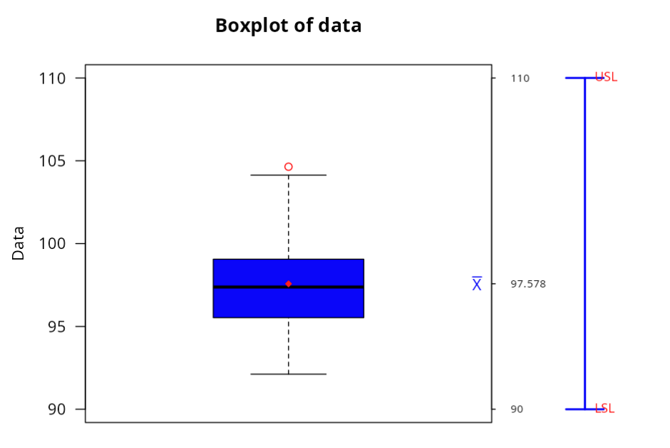
Outliers
| The Order of Collection | Data | |
|---|---|---|
| 1 | 14 | 104,64 |
Automatic Analysis
| Process Analysis | Situation | |
|---|---|---|
| 1 | Normality Test | Accept a 0.05 significance level |
| 2 | Box-Cox Transformation | No Aplicable |
| 3 | Johnson Transformation | No Aplicable |
| 4 | Non-Normal Distribution | No Aplicable |
| 5 | Non-Parametric Distribution | NO Aplicable |
Normality test
| Statistics | P-Value | |
|---|---|---|
| Anderson Darling | 0,2613 | 0,6836 |
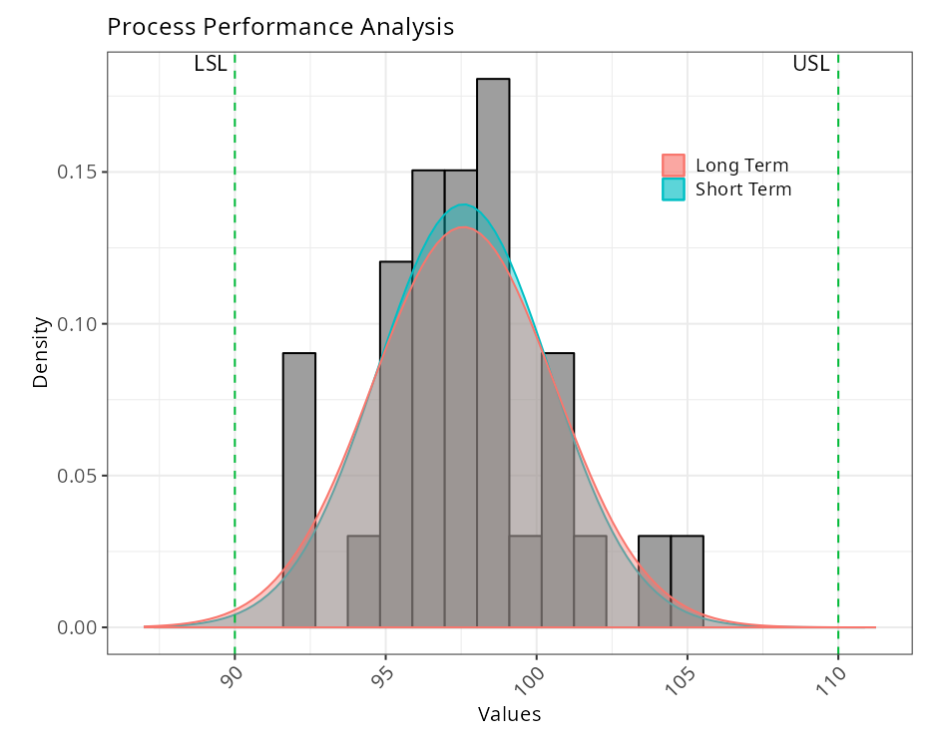
Specifications
| Value | ||
|---|---|---|
| 1 | Sample | 31 |
| 2 | Lower Limit | 90 |
| 3 | Upper Limit | 110 |
Estimates
| Value | |
|---|---|
| Mean | 97.5777 |
| Standard Desviation (Short term) | 2.8625 |
| Desviación Estándar (Long term) | 3.0247 |
Performance Indices (Long term)
| Performance Indexes - Total Variability | |
|---|---|
| PP | 1.1020 |
| PPL | 0.8351 |
| PPU | 1.3690 |
| PPK | 0.8351 |
Capacity Indices (short term)
| Capacity Indices - Inherent Variability | |
|---|---|
| CP | 1.1645 |
| CPI | 0.8824 |
| CPS | 1.4465 |
| CPK | 0.8824 |
Observed Indices
| Observed Indices | |
|---|---|
| PPM < LIE | 0 |
| PPM > LSE | 0 |
| PPM Total | 0 |
Observed Indices (Long Term)
| Observed Indices (Total Variability) | |
|---|---|
| PPM < LIE | 6118.1571 |
| PPM > LSE | 20.0514 |
| PPM Total | 6138.2086 |
Expected Indexes (Short term)
| Expected Indexes (Inherent Variability) | |
|---|---|
| PPM < LSL | 4057.6342 |
| PPM > USL | 7.1359 |
| PPM Total | 4064.7701 |
SIGMA LEVEL
| SIGMA Level | |
|---|---|
| Zbench (long term) | 2.5041 |
| Zbench (short term) | 2.6466 |
| Zshift | 1.5 |
| Sigma Metrics | 4.0041 |
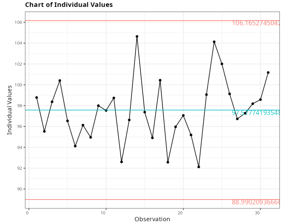
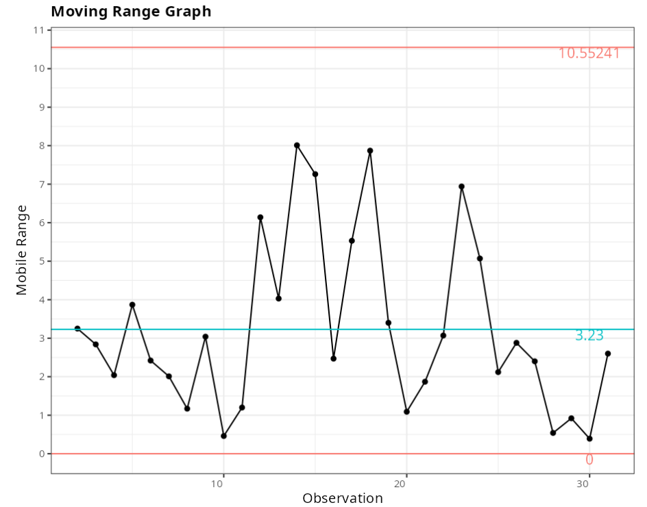
Análisis Gráfico
Estabilidad del Proceso
Gráfico de Valores Individuales y Amplitudes móviles
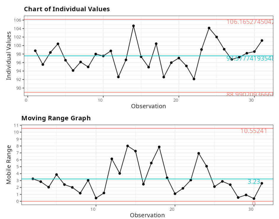
Individual Values Chart
| Valor | |
|---|---|
| Lower Control Limit | 88.9902 |
| Center line | 97.5777 |
| Upper Control Limit | 106.1653 |
Moving Range Chart
| Value | |
|---|---|
| Lower Control Limit | 0 |
| Center Line | 3.23 |
| Upper Control Limit | 10.5524 |
Example 2:
An analyst measured the weight in mg/pill of a substance for 30 lots divided into subgroups of size 3. The specifications LEL = 173 mg and LSE = 187 mg have been defined. The aim is to generate a complete statistical report to review the process:
| Lots | Weight |
|---|---|
| 2024001 | 174.8 |
| 2024001 | 176.7 |
| 2024001 | 176.6 |
| 2024002 | 177.7 |
| 2024002 | 181.2 |
| 2024002 | 181.9 |
| 2024003 | 180.3 |
| 2024003 | 179.8 |
| 2024003 | 179 |
| 2024004 | 176.3 |
| 2024004 | 178.5 |
| 2024004 | 180.1 |
| 2024005 | 179.6 |
| 2024005 | 180.6 |
| 2024005 | 178.8 |
| 2024006 | 174.4 |
| 2024006 | 177.4 |
| 2024006 | 178.8 |
| 2024007 | 176.3 |
| 2024007 | 178 |
| 2024007 | 179.6 |
| 2024008 | 180 |
| 2024008 | 179.2 |
| 2024008 | 177.4 |
| 2024009 | 178.1 |
| 2024009 | 178.1 |
| 2024009 | 179.3 |
| 2024010 | 179.3 |
| 2024010 | 181.5 |
| 2024010 | 178.4 |
| 2024011 | 180.9 |
| 2024011 | 180.6 |
| 2024011 | 179.5 |
| 2024012 | 178.7 |
| 2024012 | 178.6 |
| 2024012 | 179.8 |
| 2024013 | 175.3 |
| 2024013 | 180.0 |
| 2024013 | 178.0 |
| 2024014 | 179.8 |
| 2024014 | 180.7 |
| 2024014 | 181.2 |
| 2024015 | 181.0 |
| 2024015 | 178.2 |
| 2024015 | 176.5 |
| 2024016 | 176.4 |
| 2024016 | 176.5 |
| 2024016 | 178.4 |
| 2024017 | 184.8 |
| 2024017 | 183.2 |
| 2024017 | 177.6 |
| 2024018 | 176.9 |
| 2024018 | 176.0 |
| 2024018 | 177.0 |
| 2024019 | 176.9 |
| 2024019 | 178.5 |
| 2024019 | 178.9 |
| 2024020 | 177.4 |
| 2024020 | 177.7 |
| 2024020 | 178.6 |
| 2024021 | 180.3 |
| 2024021 | 179.4 |
| 2024021 | 179.1 |
| 2024022 | 178.3 |
| 2024022 | 176.1 |
| 2024022 | 175.0 |
| 2024023 | 176.2 |
| 2024023 | 179.9 |
| 2024023 | 181.1 |
| 2024024 | 178.2 |
| 2024024 | 179.4 |
| 2024024 | 178.5 |
| 2024025 | 178.3 |
| 2024025 | 176.9 |
| 2024025 | 178.0 |
| 2024026 | 180.6 |
| 2024026 | 177.0 |
| 2024026 | 176.8 |
| 2024027 | 178.0 |
| 2024027 | 178.6 |
| 2024027 | 179.8 |
| 2024028 | 178.5 |
| 2024028 | 180.6 |
| 2024028 | 179.2 |
| 2024029 | 179.1 |
| 2024029 | 176.9 |
| 2024029 | 177.6 |
| 2024030 | 177.5 |
| 2024030 | 178.0 |
| 2024030 | 178.5 |
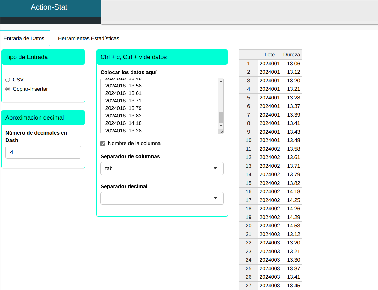
We will upload the data to the system.
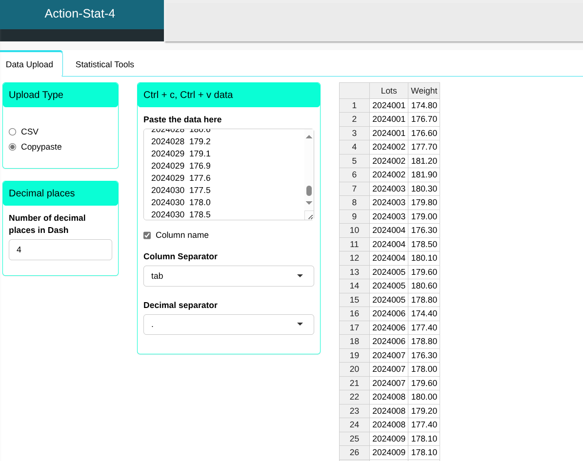
Configuring as shown in the figure below to perform the analysis.
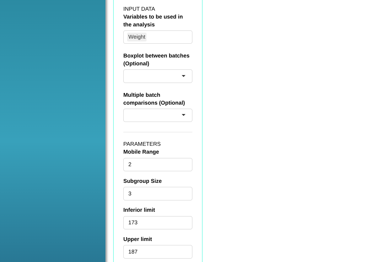

Then click Calculate we obtain the results. You can also generate the analyses and download them in Word format.
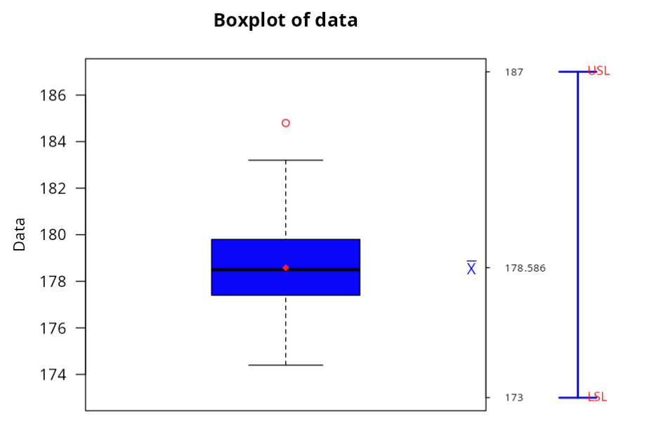
The results are:
Descriptive summary
| Statistics | |
|---|---|
| Minimum | 174.4 |
| 1º Quartile | 177.4 |
| Meana | 178.5856 |
| Median | 178.5 |
| Tri-Mean | 178.5486 |
| 3º Quartile | 179.8 |
| Maximum | 184.8 |
| Standard Desviation | 1.8197 |
| Coefficient of Variation (%) | 1.0189 |
| Asymmetry | 0.3461 |
| Kurtosis | 0.6338 |
| Range | 10.4 |
| Sample Size | 90 |
Outliers
| The Order of Collection | Data | |
|---|---|---|
| 1 | 17 | 184.8 |
Automatic Analysis
| Process Analysis | Situation | |
|---|---|---|
| 1 | Normality Test | Accept a 0.05 significance level |
| 2 | Box-Cox Transformation | No Aplicable |
| 3 | Johnson Transformation | No Aplicable |
| 4 | Non-Normal Distribution | No Aplicable |
| 5 | Non-Parametric | No Aplicable |
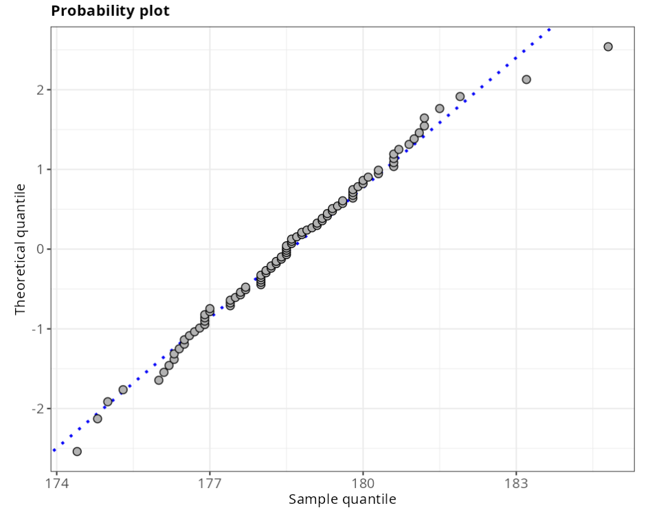
Normality tests
| Estatistics | P-values | |
|---|---|---|
| Anderson Darling | 0.2273 | 0.8093 |
Specifications
| Value | ||
|---|---|---|
| 1 | Sample | 90 |
| 2 | Lower Limit | 173 |
| 3 | Upper Limit | 187 |
Estimates
| Value | |
|---|---|
| Mean | 178.5856 |
| Standard Desviation (Short term) | 1.5184 |
| Standard Desviation (Long term) | 1.8197 |
Performance Indexes (Long term)
| Performance Indexes (Total Variability) | |
|---|---|
| PP | 1.2823 |
| PPL | 1.0232 |
| PPU | 1.5414 |
| PPK | 1.0232 |
Capacity Indexes (Short term)
| Capacity Indexes (Inherent Variability) | |
|---|---|
| CP | 1.5367 |
| CPI | 1.2262 |
| CPS | 1.8472 |
| CPK | 1.2262 |
Observed Indices
| Observed Indices | |
|---|---|
| PPM < LSL | 0 |
| PPM > USL | 0 |
| PPM Total | 0 |
Expected Indexes (Long term)
| Expected Indexes (Total Variability) | |
|---|---|
| PPM < LSL | 1071.8298 |
| PPM > USL | 1.8802 |
| PPM Total | 1073.7100 |
Expected Indexes (Short term)
| Expected Indexes (Inherent Variability) | |
|---|---|
| PPM < LSL | 117.2693 |
| PPM > USL | 0.0150 |
| PPM Total | 117.2843 |
SIGMA LEVEL
| SIGMA Level | |
|---|---|
| Zbench (long term) | 3.069 |
| Zbench (short term) | 3.6785 |
| Zshift | 1.5 |
| Sigma Metrics | 4.569 |
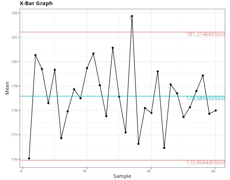
Análisis Gráfico
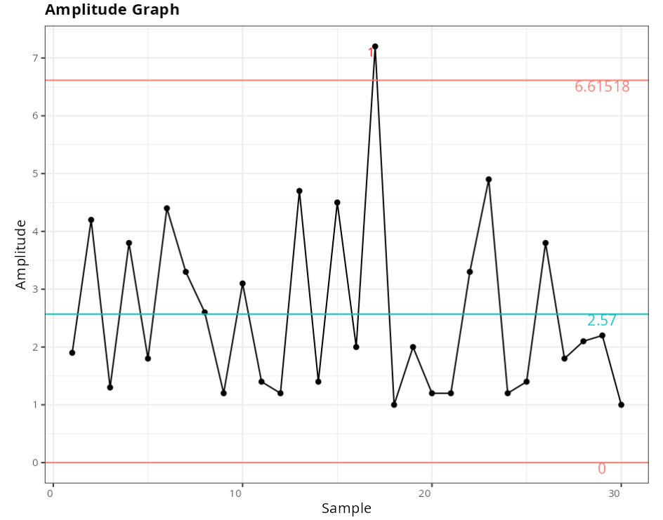
Process Stability - Mean and Range Graphs
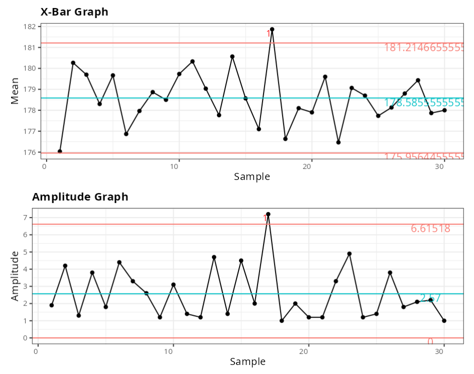
Xbar Graph
| Value | |
|---|---|
| Lower Control Limit | 175.9564 |
| Center Line | 178.5856 |
| Upper Control Limit | 181.2147 |
Range Chart
| Value | |
|---|---|
| Lower Control Limit | 0 |
| Center Line | 2.57 |
| Upper Control Limit | 6.6152 |
Example 3:
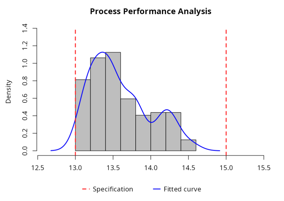
An analyst has measured the weight in mg/pill of a substance for 10 lots, divided into subgroups of size 10. The specifications LSL = 13 and USL = 15 have been defined. The aim is to generate a complete statistical report to review the process:
| Lot | Hardness | Lot | Hardness |
|---|---|---|---|
| 2024001 | 13.06 | 2024009 | 13.61 |
| 2024001 | 13.12 | 2024009 | 13.71 |
| 2024001 | 13.20 | 2024009 | 13.79 |
| 2024001 | 13.21 | 2024009 | 13.82 |
| 2024001 | 13.28 | 2024009 | 14.18 |
| 2024001 | 13.37 | 2024009 | 14.25 |
| 2024001 | 13.39 | 2024009 | 14.26 |
| 2024001 | 13.41 | 2024009 | 14.29 |
| 2024001 | 13.43 | 2024009 | 14.53 |
| 2024001 | 13.48 | 2024009 | 13.12 |
| 2024002 | 13.58 | 2024010 | 13.20 |
| 2024002 | 13.61 | 2024010 | 13.21 |
| 2024002 | 13.71 | 2024010 | 13.30 |
| 2024002 | 13.79 | 2024010 | 13.37 |
| 2024002 | 13.82 | 2024010 | 13.41 |
| 2024002 | 14.18 | 2024010 | 13.45 |
| 2024002 | 14.25 | 2024010 | 13.53 |
| 2024002 | 14.26 | 2024010 | 13.57 |
| 2024002 | 14.29 | 2024010 | 13.80 |
| 2024002 | 14.53 | 2024010 | 13.81 |
| 2024003 | 13.12 | 2024011 | 13.82 |
| 2024003 | 13.20 | 2024011 | 14.09 |
| 2024003 | 13.21 | 2024011 | 13.06 |
| 2024003 | 13.30 | 2024011 | 13.12 |
| 2024003 | 13.37 | 2024011 | 13.20 |
| 2024003 | 13.41 | 2024011 | 13.21 |
| 2024003 | 13.45 | 2024011 | 13.28 |
| 2024003 | 13.53 | 2024011 | 13.37 |
| 2024003 | 13.57 | 2024011 | 13.39 |
| 2024003 | 13.80 | 2024011 | 13.41 |
| 2024004 | 13.81 | 2024012 | 13.43 |
| 2024004 | 13.82 | 2024012 | 13.48 |
| 2024004 | 14.09 | 2024012 | 13.58 |
| 2024004 | 14.13 | 2024012 | 13.61 |
| 2024004 | 14.18 | 2024012 | 13.71 |
| 2024004 | 14.35 | 2024012 | 13.79 |
| 2024004 | 13.06 | 2024012 | 13.82 |
| 2024004 | 13.12 | 2024012 | 14.18 |
| 2024004 | 13.20 | 2024012 | 14.25 |
| 2024004 | 13.21 | 2024012 | 14.26 |
| 2024005 | 13.37 | 2024013 | 14.29 |
| 2024005 | 13.39 | 2024013 | 14.53 |
| 2024005 | 13.41 | 2024013 | 13.12 |
| 2024005 | 13.43 | 2024013 | 13.20 |
| 2024005 | 13.48 | 2024013 | 13.21 |
| 2024005 | 13.58 | 2024013 | 13.3 |
| 2024005 | 13.61 | 2024013 | 13.37 |
| 2024005 | 13.71 | 2024013 | 13.41 |
| 2024005 | 13.79 | 2024013 | 13.45 |
| 2024005 | 13.82 | 2024013 | 13.53 |
| 2024006 | 14.18 | 2024014 | 13.57 |
| 2024006 | 14.25 | 2024014 | 13.80 |
| 2024006 | 14.26 | 2024014 | 13.81 |
| 2024006 | 14.29 | 2024014 | 13.82 |
| 2024006 | 14.53 | 2024014 | 14.09 |
| 2024006 | 13.12 | 2024014 | 14.13 |
| 2024006 | 13.20 | 2024014 | 14.18 |
| 2024006 | 13.21 | 2024014 | 14.35 |
| 2024006 | 13.30 | 2024014 | 13.06 |
| 2024006 | 13.37 | 2024014 | 13.12 |
| 2024007 | 13.41 | 2024015 | 13.20 |
| 2024007 | 13.45 | 2024015 | 13.21 |
| 2024007 | 13.53 | 2024015 | 13.28 |
| 2024007 | 13.57 | 2024015 | 13.06 |
| 2024007 | 13.80 | 2024015 | 13.12 |
| 2024007 | 13.81 | 2024015 | 13.20 |
| 2024007 | 13.82 | 2024015 | 13.21 |
| 2024007 | 14.09 | 2024015 | 13.28 |
| 2024007 | 14.13 | 2024015 | 13.37 |
| 2024007 | 13.06 | 2024015 | 13.39 |
| 2024008 | 13.12 | 2024016 | 13.41 |
| 2024008 | 13.20 | 2024016 | 13.43 |
| 2024008 | 13.21 | 2024016 | 13.48 |
| 2024008 | 13.28 | 2024016 | 13.58 |
| 2024008 | 13.37 | 2024016 | 13.61 |
| 2024008 | 13.39 | 2024016 | 13.71 |
| 2024008 | 13.41 | 2024016 | 13.79 |
| 2024008 | 13.43 | 2024016 | 13.82 |
| 2024008 | 13.48 | 2024016 | 14.18 |
| 2024008 | 13.58 | 2024016 | 13.28 |
We will upload the data to the system.
Configuring as shown in the figure below to perform the analysis.

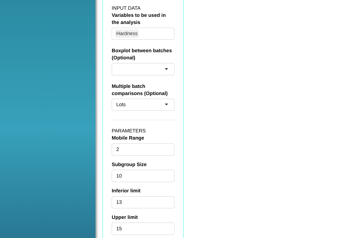
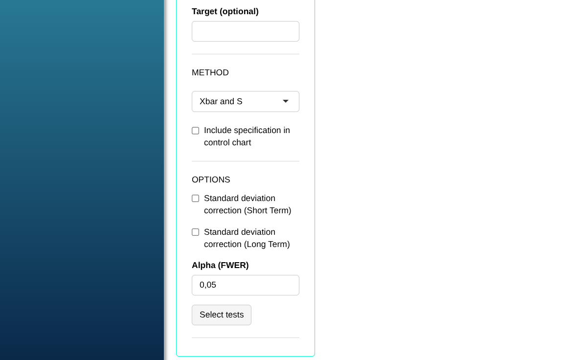
Then click Calculate we obtain the results. You can also generate the analyses and download them in Word format.
The results are:
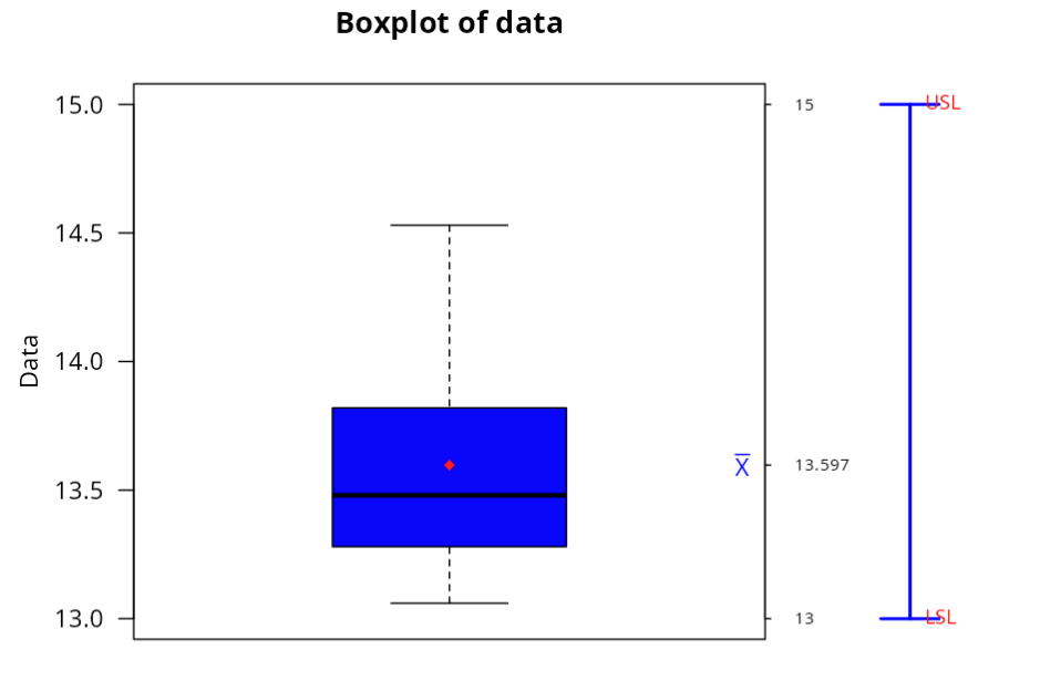
Descriptive summary
| Statistics | |
|---|---|
| Minimum | 13.06 |
| 1º Quartile | 13.28 |
| Mean | 13.5972 |
| Median | 13.48 |
| Tri-Mean | 13.5662 |
| 3º Quartile | 13.82 |
| Maximum | 14.53 |
| Standard Desviation | 0.3933 |
| Coefficient of Variation (%) | 2.8924 |
| Asymmetry | 0.6638 |
| Kurtosis | -0.6347 |
| Range | 1.47 |
| Sample Size | 160 |
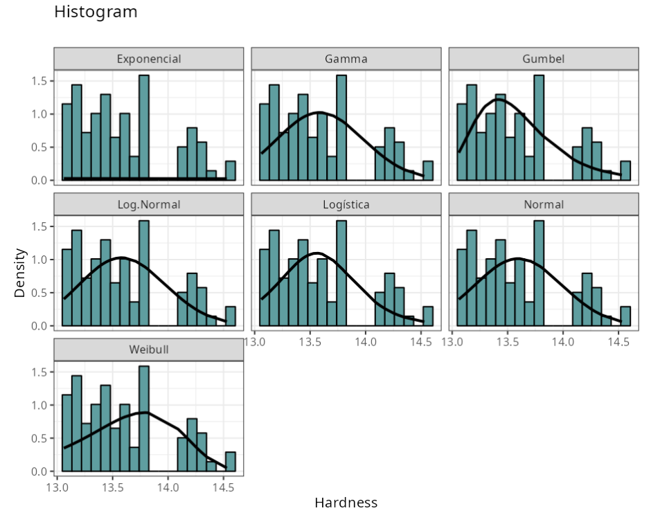
Automatic Analysis
| Process Analysis | Situation | |
|---|---|---|
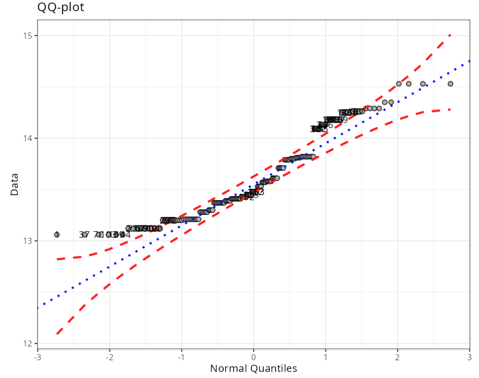
| 1 | Normality Test | Normality hypothesis rejected at 5% significance level |
| 2 | Box-Cox Transformation | Could not use Box-cox transformation |
| 3 | Johnson Transformation | Could not use Johnson transformation |
| 4 | Non-Normal Distribution | It was not possible to use other parametric distribution |
| 5 | Non-Parametric Distribution | The Kernel nonparametric method was used for the adjustment of the them. |
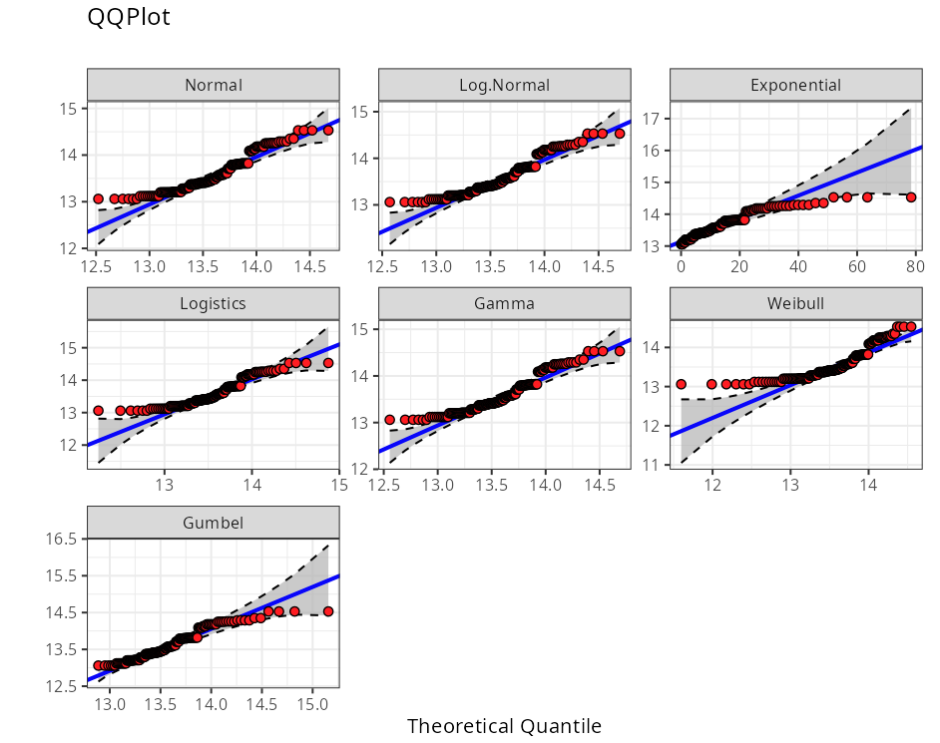
Anderson-Darling
| Distribution | Statistics | P-value |
|---|---|---|
| Normal($\mu$ = 13.6, $\sigma$ = 0.39) | 4.3496 | 0.0000 |
| Log-Normal(log($\mu$) = 2.60946, log($\sigma$) = 0.0285766) | 4.0776 | 0.0000 |
| Exponencial(Tasa = 0.0735443) | 69.3914 | 0.0000 |
| Logística(Posición = 13.56, Escala = 0.23) | 3.8440 | 0.0050 |
| Gamma(Shape = 1217.62, Rate = 89.5491) | 4.1954 | 0.0050 |
| Weibull(Shape = 33.1981, Scale = 13.7979) | 7.0015 | 0.0100 |
| Gumbel(Location = 13.416, Scale = 0.301584) | 2.0802 | 0.0100 |
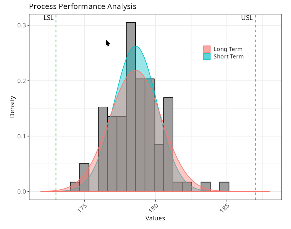
Process stability
Specification
| Value | ||
|---|---|---|
| 1 | Sample | 160 |
| 2 | Lower Limit | 13 |
| 3 | Upper Limit | 15 |
Estimates
| Parameters | Value | |
|---|---|---|
| 1 | Mean | 13.59725 |
| 2 | Standard Desviation | 0.393291144736697 |
Performance Indexes
| Performance Indexes | ||
|---|---|---|
| 1 | PP | 1.0353 |
| 2 | PPL | 0.7232 |
| 3 | PPU | 1.2156 |
| 4 | PPK | 0.7232 |
Observed Indices
| Observed Indices | ||
|---|---|---|
| 1 | PPM > USL | 0 |
| 2 | PPM < LSL | 0 |
Expected Indexes
| Expected Indexes | ||
|---|---|---|
| 1 | PPM > USL | 0 |
| 2 | PPM < LSL | 30774.1006085405 |
| 3 | PPM Total | 30774.1006085405 |
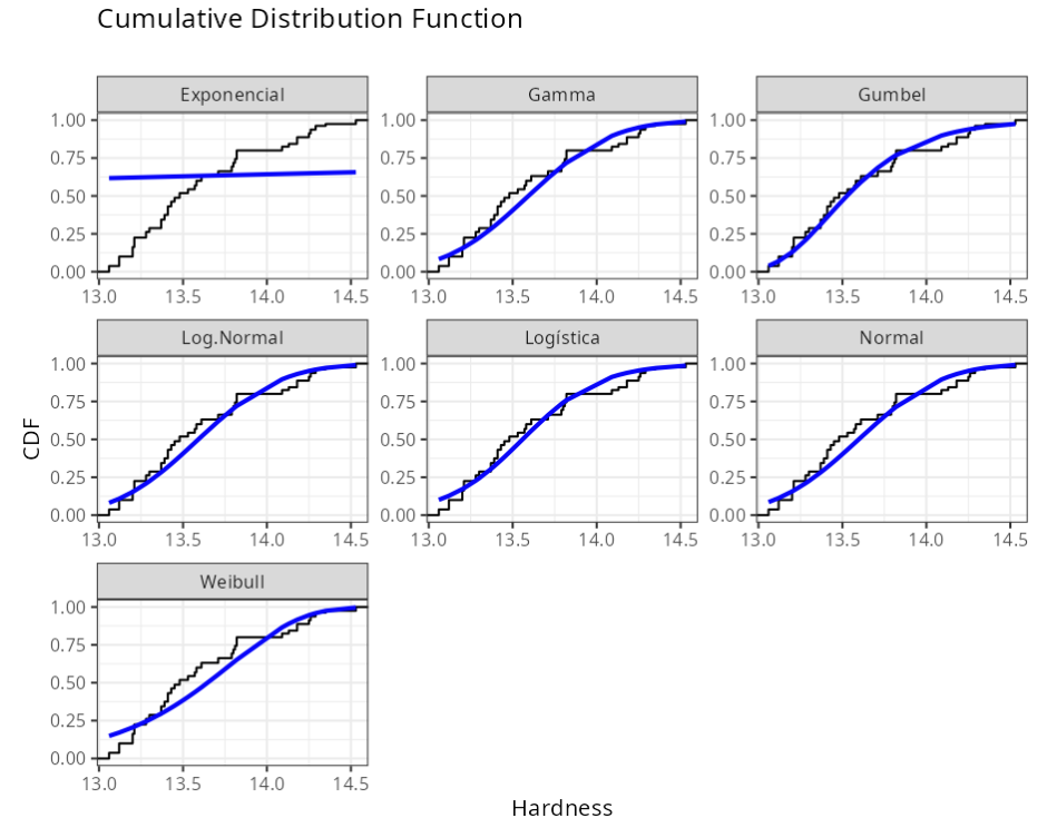
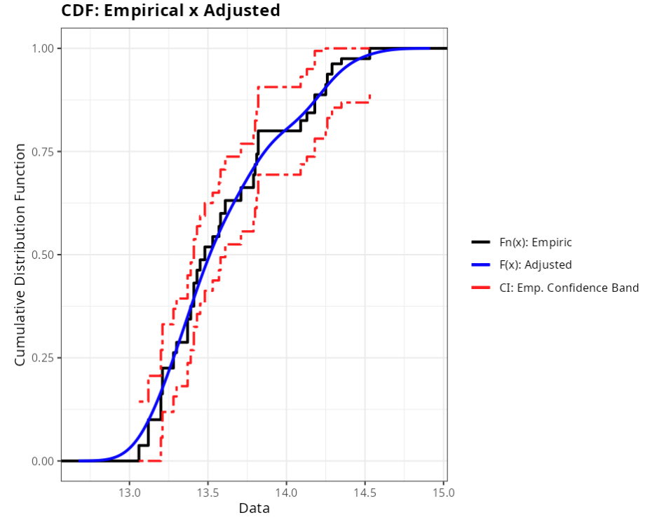
Fit Quality (Non-Parametric (Core): Method gaussian)
| Method | Statistic | P-value | |
|---|---|---|---|
| Cramér-von Mises | gaussian | 0.0929 | 0.7652 |
| Kolmogorov-Smirnov | gaussian | 0.0750 | 0.7591 |
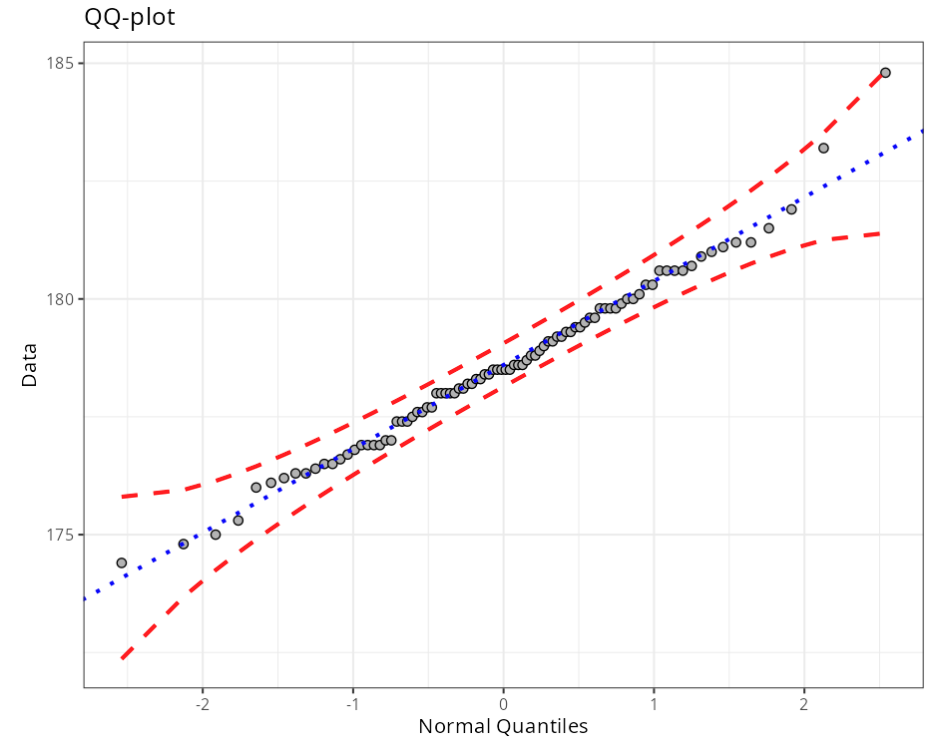
Normality Test (Outliers)
| Obs. | Normal Quantiles | Data | Criterion | |
|---|---|---|---|---|
| 1 | 1 | -2.73 | 13.06 | Envelope (Confidence Level=95%) |
| 2 | 43 | -2.35 | 13.06 | Envelope (Confidence Level=95%) |
| 3 | 63 | -2.15 | 13.06 | Envelope (Confidence Level=95%) |
| 4 | 100 | -2.02 | 13.06 | Envelope (Confidence Level=95%) |
| 5 | 142 | -1.91 | 13.06 | Envelope (Confidence Level=95%) |
| 6 | 151 | -1.82 | 13.06 | Envelope (Confidence Level=95%) |
| 7 | 3 | -1.74 | 13.12 | Envelope (Confidence Level=95%) |
| 8 | 8 | -1.68 | 13.12 | Envelope (Confidence Level=95%) |
| 9 | 17 | -1.62 | 13.12 | Envelope (Confidence Level=95%) |
| 10 | 45 | -1.56 | 13.12 | Envelope (Confidence Level=95%) |
| 11 | 59 | -1.51 | 13.12 | Envelope (Confidence Level=95%) |
| 12 | 79 | -1.46 | 13.12 | Envelope (Confidence Level=95%) |
| 13 | 86 | -1.42 | 13.12 | Envelope (Confidence Level=95%) |
| 14 | 116 | -1.38 | 13.12 | Envelope (Confidence Level=95%) |
| 15 | 10 | -1.26 | 13.2 | Envelope (Confidence Level=95%) |
| 16 | 15 | -1.23 | 13.2 | Envelope (Confidence Level=95%) |
| 17 | 19 | -1.20 | 13.2 | Envelope (Confidence Level=95%) |
| 18 | 24 | -1.17 | 13.2 | Envelope (Confidence Level=95%) |
| 19 | 33 | -1.14 | 13.2 | Envelope (Confidence Level=95%) |
| 20 | 27 | 0.85 | 14.09 | Envelope (Confidence Level=95%) |
| 21 | 36 | 0.88 | 14.09 | Envelope (Confidence Level=95%) |
| 22 | 78 | 0.90 | 14.09 | Envelope (Confidence Level=95%) |
| 23 | 119 | 0.92 | 14.09 | Envelope (Confidence Level=95%) |
| 24 | 52 | 0.95 | 14.13 | Envelope (Confidence Level=95%) |
| 25 | 94 | 0.97 | 14.13 | Envelope (Confidence Level=95%) |
| 26 | 135 | 1.00 | 14.13 | Envelope (Confidence Level=95%) |
| 27 | 6 | 1.02 | 14.18 | Envelope (Confidence Level=95%) |
| 28 | 68 | 1.05 | 14.18 | Envelope (Confidence Level=95%) |
| 29 | 73 | 1.08 | 14.18 | Envelope (Confidence Level=95%) |
| 30 | 82 | 1.11 | 14.18 | Envelope (Confidence Level=95%) |
| 31 | 110 | 1.14 | 14.18 | Envelope (Confidence Level=95%) |
| 32 | 124 | 1.17 | 14.18 | Envelope (Confidence Level=95%) |
| 33 | 144 | 1.20 | 14.18 | Envelope (Confidence Level=95%) |
| 34 | 22 | 1.23 | 14.25 | Envelope (Confidence Level=95%) |
| 35 | 89 | 1.26 | 14.25 | Envelope (Confidence Level=95%) |
| 36 | 98 | 1.30 | 14.25 | Envelope (Confidence Level=95%) |
| 37 | 140 | 1.34 | 14.25 | Envelope (Confidence Level=95%) |
| 38 | 38 | 1.38 | 14.26 | Envelope (Confidence Level=95%) |
| 39 | 105 | 1.42 | 14.26 | Envelope (Confidence Level=95%) |
| 40 | 114 | 1.46 | 14.26 | Envelope (Confidence Level=95%) |
| 41 | 129 | -0.10 | 13.43 | Envelope (Confidence Level=95%) |
| 42 | 99 | -0.05 | 13.45 | Envelope (Confidence Level=95%) |
| 43 | 141 | -0.04 | 13.45 | Envelope (Confidence Level=95%) |
| 44 | 136 | 0.02 | 13.48 | Envelope (Confidence Level=95%) |
| 45 | 145 | 0.04 | 13.48 | Envelope (Confidence Level=95%) |
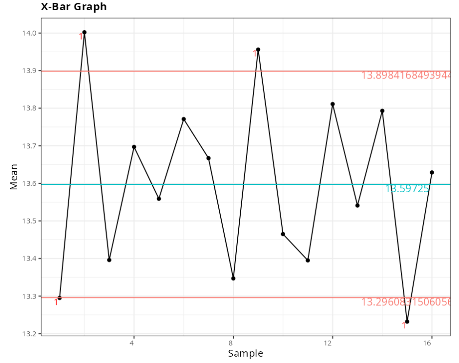
Process stability
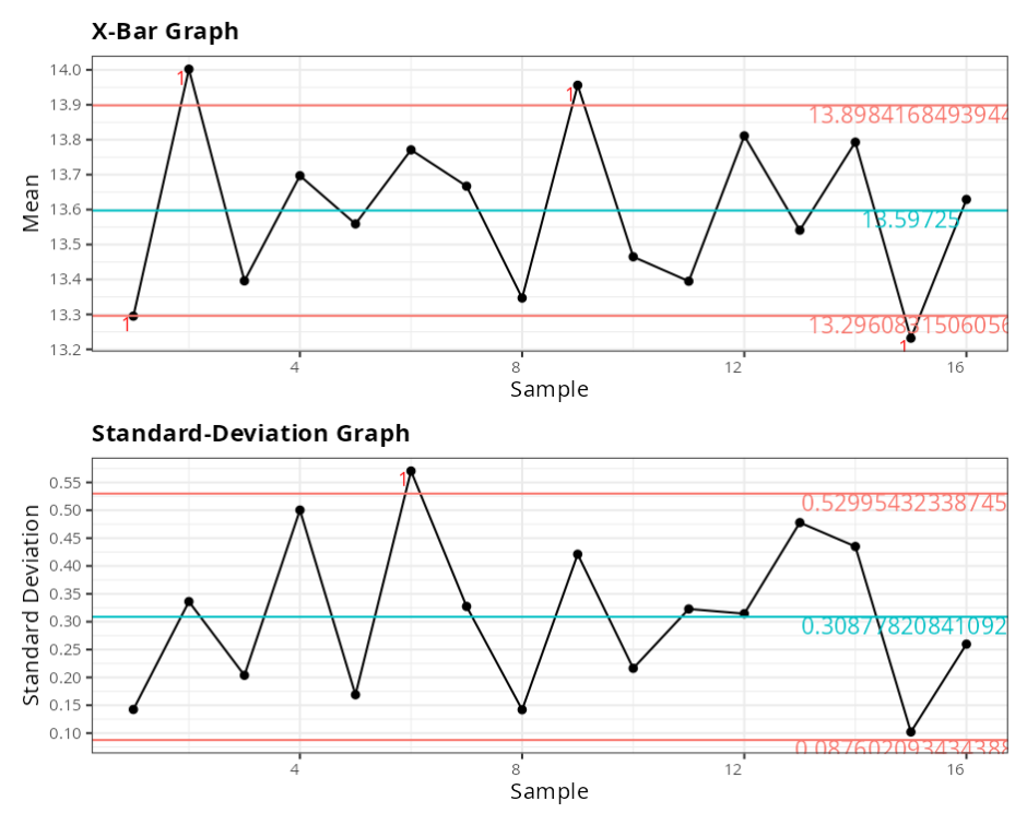
Xbar Graph
| Value | |
|---|---|
| Lower Control Limit | 13.2961 |
| Center Line | 13.5972 |
| Upper control Limit | 13.8984 |
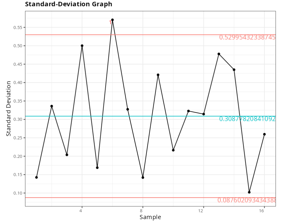
Standard Deviation graph
| Value | |
|---|---|
| Lower Control Limit | 0.0876 |
| Center Line | 0.3088 |
| Upper Control Limit | 0.53 |
Kruskal-Wallis test
| Value | |
|---|---|
| Statistics | 54.2338 |
| Degrees of Freedom | 15 |
| P-value | 0 |
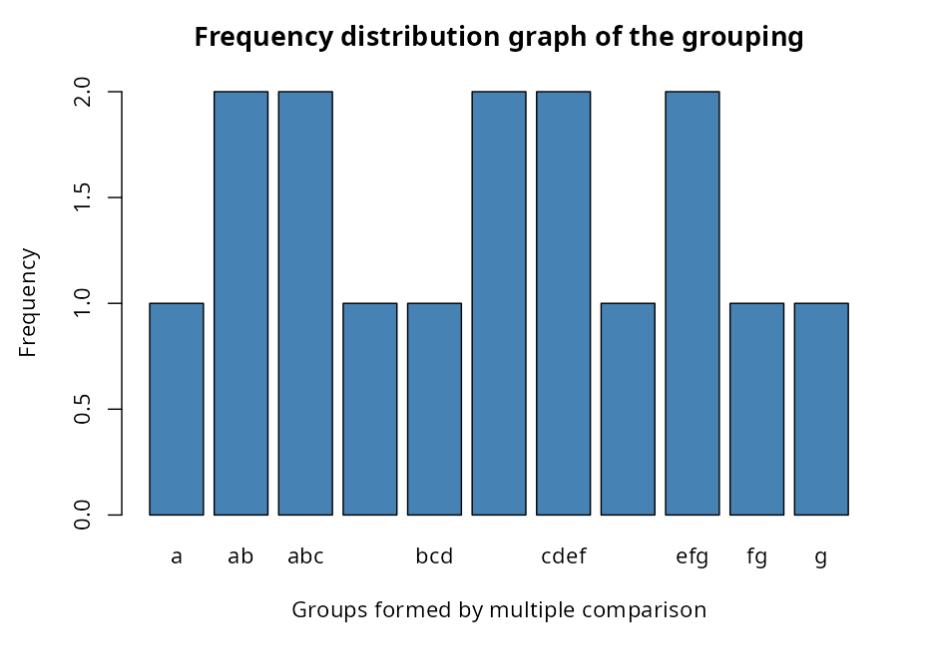
Table of Grouped comparison of Groups (Kruskal Wallis)
| Factor | Mean | Median | Mean ofyhe Ranks | Groups |
|---|---|---|---|---|
| 2024002 | 14.0020 | 14.0000 | 127.3000 | a |
| 2024009 | 13.9560 | 14.0000 | 119.0500 | ab |
| 2024012 | 13.8110 | 13.7500 | 111.5000 | ab |
| 2024014 | 13.7930 | 13.8150 | 101.8500 | abc |
| 2024007 | 13.6670 | 13.6850 | 93.9500 | abc |
| 2024016 | 13.6290 | 13.5950 | 92.6500 | abcd |
| 2024006 | 13.7710 | 13.7750 | 90.3000 | bcd |
| 2024004 | 13.6970 | 13.8150 | 86.8500 | bcde |
| 2024005 | 13.5590 | 13.5300 | 85.7000 | bcde |
| 2024013 | 13.5410 | 13.3900 | 69.8000 | cdef |
| 2024010 | 13.4650 | 13.4300 | 69.6000 | cdef |
| 2024003 | 13.3960 | 13.3900 | 59.0000 | defg |
| 2024011 | 13.3950 | 13.3250 | 53.6000 | efg |
| 2024008 | 13.3470 | 13.3800 | 52.5000 | efg |
| 2024001 | 13.2950 | 13.3250 | 43.4500 | fg |
| 2024015 | 13.2320 | 13.2100 | 30.9000 | g |
Table Proportion of Total Groups Formed by the Total of Lots
| Valores | |
|---|---|
| Number of groups Formed | 11 |
| Total Frequency | 16 |
| Proportion of Groups by the Total of Lots | 68.75 |