3. Analysis by Period
ANVISA guidance requires the various pharmaceutical industries to carry out a statistical evaluation of the results of in-process and finished product control. The methodology presented here is well-founded and follows the requirements of the ANVISA Guide (2012). Action Stat provides a statistical tool that allows the generation of complete product quality analysis reports, containing a statistical methodology that follows the following flow: first, an exploratory analysis of the results is carried out with a descriptive summary and a BoxPlot graph. This is followed by a distribution fit test. Next, the stability of the process is assessed using control charts. This is followed by an assessment of the capacity and performance of the process and, finally, a multiple lots comparison test.
Analysis by Period
Period analysis is used when you want to compare control analyses for a given period.
Example 1:
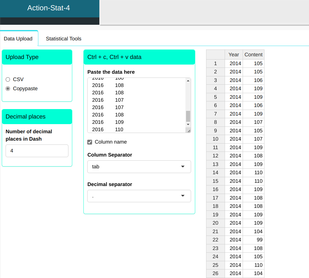
An analyst measured the content of a substance over three years: 2014, 2015 and 2016. The specifications were defined as LSL = 90 and USL = 110. The objective is to generate a complete statistical analysis report by period:
| Year | Content | year | Content | year | Content |
|---|---|---|---|---|---|
| 2014 | 105 | 2015 | 107 | 2016 | 109 |
| 2014 | 105 | 2015 | 107 | 2016 | 109 |
| 2014 | 106 | 2015 | 105 | 2016 | 108 |
| 2014 | 109 | 2015 | 104 | 2016 | 104 |
| 2014 | 109 | 2015 | 107 | 2016 | 105 |
| 2014 | 106 | 2015 | 108 | 2016 | 109 |
| 2014 | 109 | 2015 | 108 | 2016 | 108 |
| 2014 | 107 | 2015 | 109 | 2016 | 107 |
| 2014 | 105 | 2015 | 95 | 2016 | 98 |
| 2014 | 107 | 2015 | 101 | 2016 | 97 |
| 2014 | 109 | 2015 | 97 | 2016 | 106 |
| 2014 | 108 | 2015 | 92 | 2016 | 107 |
| 2014 | 109 | 2015 | 103 | 2016 | 105 |
| 2014 | 110 | 2015 | 99 | 2016 | 105 |
| 2014 | 110 | 2015 | 98 | 2016 | 106 |
| 2014 | 109 | 2015 | 98 | 2016 | 105 |
| 2014 | 108 | 2015 | 109 | 2016 | 108 |
| 2014 | 108 | 2015 | 108 | 2016 | 109 |
| 2014 | 109 | 2015 | 108 | 2016 | 109 |
| 2014 | 109 | 2015 | 102 | 2016 | 101 |
| 2014 | 104 | 2015 | 109 | 2016 | 101 |
| 2014 | 99 | 2016 | 109 | 2016 | 100 |
| 2014 | 108 | 2016 | 96 | 2016 | 108 |
| 2014 | 105 | 2016 | 108 | 2016 | 108 |
| 2014 | 110 | 2016 | 108 | 2016 | 107 |
| 2014 | 104 | 2016 | 105 | 2016 | 107 |
| 2015 | 106 | 2016 | 108 | 2016 | 108 |
| 2015 | 108 | 2016 | 108 | 2016 | 109 |
| 2015 | 110 | 2016 | 109 | 2016 | 110 |
| 2015 | 109 | 2016 | 109 |
We will upload the data to the system.
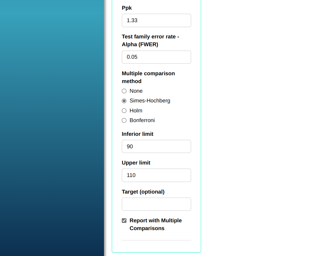
Configuring as shown in the figure below to perform the analysis.
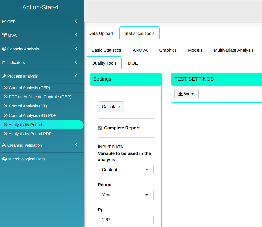
Then click Calculate we obtain the results. You can also generate the analyses and download them in Word format.

The results are:
Descriptive Analysis by Period
| 2014 | 2015 | 2016 | |
|---|---|---|---|
| Minimun | 0.99 | 0.92 | 0.96 |
| 1º Quartile | 1.05 | 1 | 1.05 |
| Mean | 1.0719 | 1.0428 | 1.0613 |
| Median | 1.08 | 1.07 | 1.08 |
| 3º Quartile | 1.09 | 1.08 | 1.09 |
| Maximum | 1.1 | 1.1 | 1.1 |
| Standard Deviation | 0.0255 | 0.0513 | 36 |
| Coefficient of Variation | 2.3751 | 4.9172 | 3.3949 |
| Asymmetry | -1.2695 | -0.83 | -1417 |
| Kurtosis | 1.6527 | -0.6171 | 1.0048 |
| Range | 0.11 | 0.18 | 0.14 |
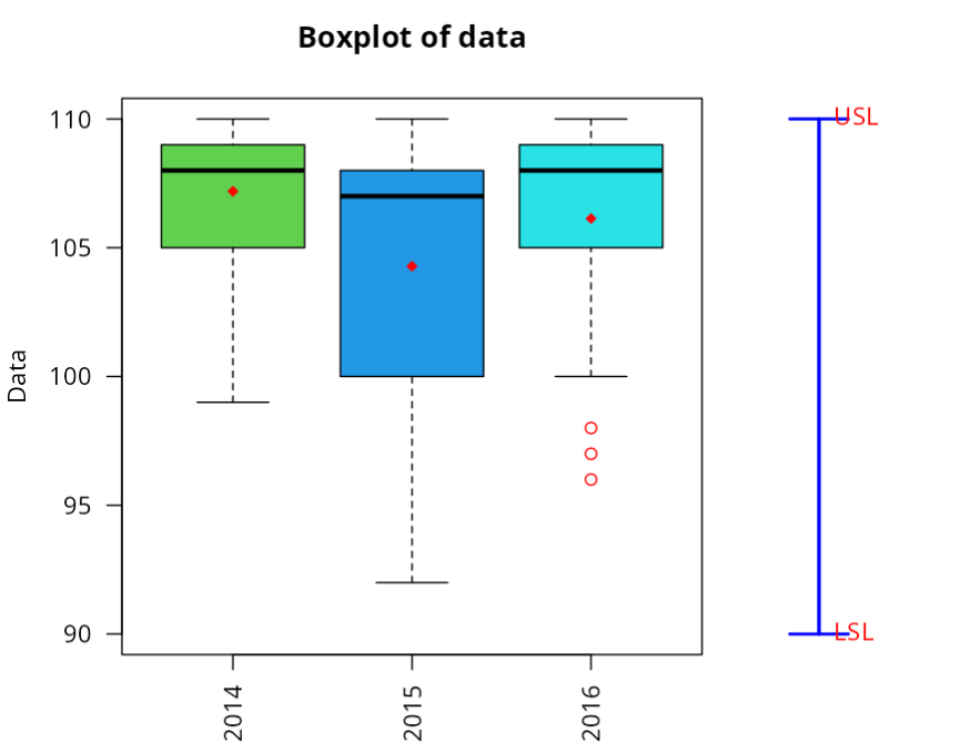
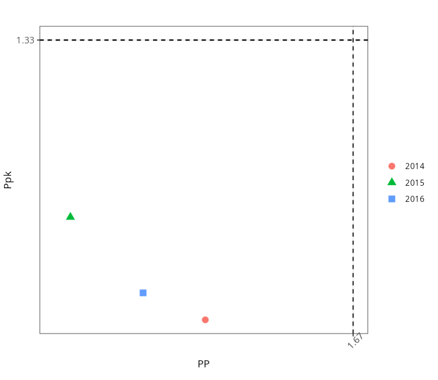
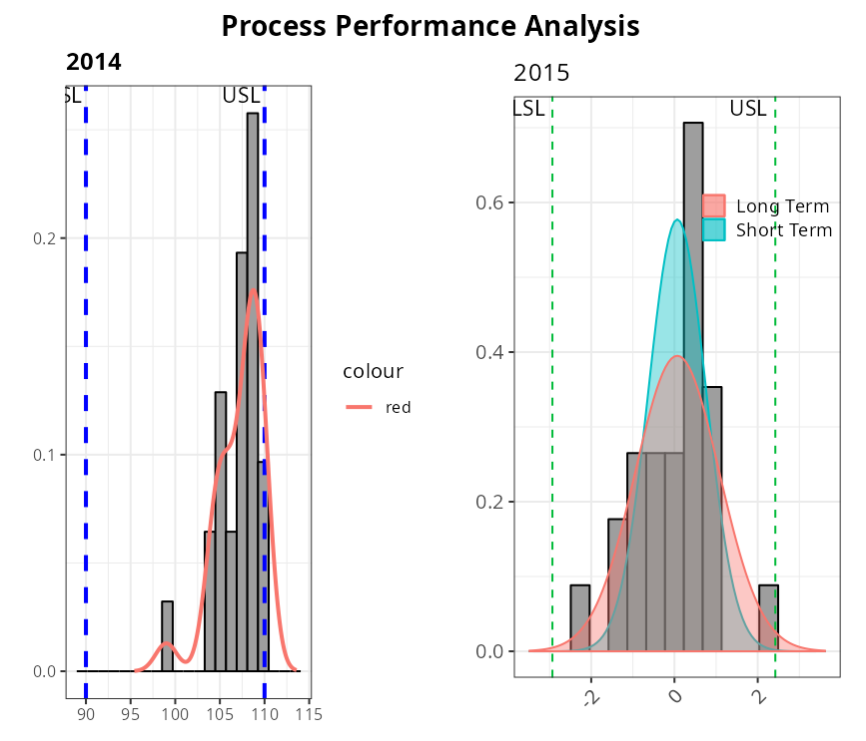
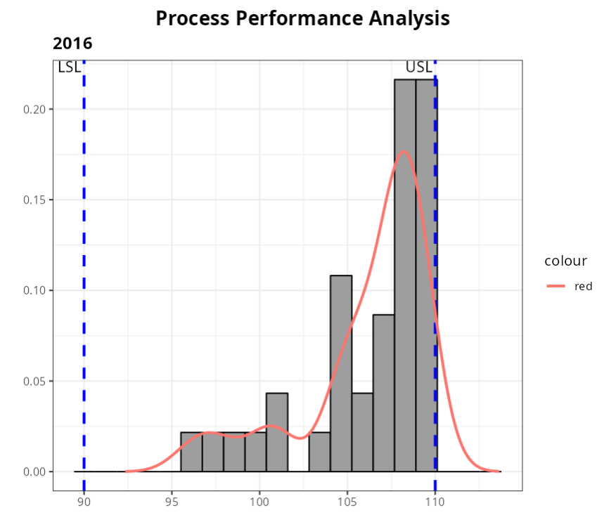
Table of Performance Indices
| 2014 | 2015 | 2016 | |
|---|---|---|---|
| PP | 1.2590 | 0.8840 | 1.0860 |
| PPL | 1.6328 | 0.9905 | 1.2980 |
| PPU | 0.4570 | 0.7774 | 0.5411 |
| PPk | 0.4570 | 0.7774 | 0.5411 |
Multiple Comparison Table
| Difference in Ranks | Corrected P-value (Simes-Hochberg) | Lower Limit | Upper Limit | |
|---|---|---|---|---|
| 2014 - 2015 | $\qquad$ 15.4423 | $\qquad\qquad$ 0.0923 | 1.4649 | 29.4197 |
| 2014 - 2016 | $\qquad$ 7.2713 | $\qquad\qquad$ 0.2582 | -5.4289 | 19.9714 |
| 2015 - 2016 | $\qquad$ -8.1711 | $\qquad\qquad$ 0.2582 | -21.0211 | 4.6790 |
Table of Grouped comparison of Periods (Kurskal-Wallis)
| Factor | Mean | Median | Mean of the Ranks | Groups |
|---|---|---|---|---|
| 2014 | 107.19 | 108 | $\qquad$ 52.4423 | a |
| 2016 | 106.13 | 108 | $\qquad$ 45.1711 | a |
| 2015 | 104.28 | 107 | $\qquad$ 37.0000 | a |