2. Process Analysis (ST)
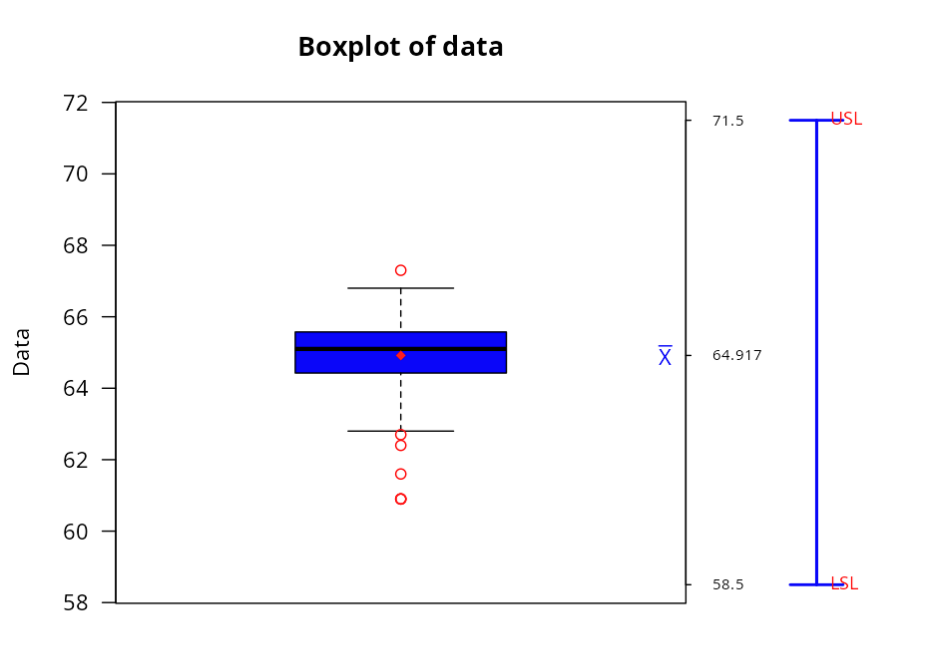
The ANVISA guidelines require that various pharmaceutical industries perform a statistical evaluation of in-process control results and finished product results. The methodology presented here is well-founded and follows the requirements of the ANVISA Guidelines (2012). Action Stat provides a statistical tool that allows for the generation of complete product quality review reports containing a statistical methodology that follows the following flow: first, an exploratory analysis of the results is performed with a descriptive summary and a BoxPlot graph. A distribution fit test is then performed. Next, process stability is evaluated using control charts. A subsequent evaluation of process capacity and performance is performed, followed by a multiple batch comparison test.
Time Series Analysis
To assess the stability of results over time, analysis using CEP charts is most often used. However, this technique is recommended only in cases where there are few subgroups of data. The recommendation is a maximum of 150 subgroups to allow for a good interpretation of the control chart. In cases where there are more than 150 subgroups, it would be best to perform the analysis using time series.
Example 1:
An analyst measured the weight of a substance for 160 production batches of a particular product over the course of a year. The specifications were defined as LSL = 58.5 mg and USL = 71.5 mg. The objective is to generate a complete statistical process review report:
| Weight |
|
|
|
|
|
|
|
| 65.5 |
65.7 |
65.5 |
65.0 |
65.4 |
65.6 |
64.6 |
65.4 |
| 64.9 |
65.5 |
64.4 |
64.5 |
64.7 |
65.1 |
64.3 |
65.4 |
| 65.7 |
65.1 |
65.5 |
64.0 |
65.1 |
65.3 |
65.0 |
65.4 |
| 65.5 |
65.6 |
65.3 |
65.1 |
64.8 |
64.7 |
65.9 |
63.8 |
| 65.8 |
64.2 |
63.8 |
65.1 |
65.3 |
64.5 |
64.4 |
61.6 |
| 63.1 |
66.8 |
65.4 |
66.5 |
66.4 |
66.0 |
63.7 |
64.9 |
| 65.2 |
66.0 |
66.2 |
65.5 |
66.0 |
66.6 |
65.8 |
65.8 |
| 64.3 |
66.8 |
65.0 |
65.3 |
65.3 |
65.3 |
65.8 |
66.0 |
| 65.8 |
65.8 |
64.6 |
66.0 |
65.5 |
64.9 |
65.9 |
65.3 |
| 63.8 |
65.6 |
64.8 |
65.0 |
65.3 |
64.8 |
65.7 |
64.1 |
| 64.7 |
65.0 |
63.3 |
64.0 |
62.9 |
64.5 |
65.0 |
63.8 |
| 65.2 |
65.1 |
64.7 |
65.1 |
65.6 |
63.4 |
66.0 |
64.4 |
| 66.0 |
64.9 |
63.8 |
64.2 |
63.1 |
65.5 |
65.2 |
66.8 |
| 66.1 |
64.9 |
65.1 |
64.9 |
60.9 |
65.2 |
64.0 |
63.5 |
| 66.3 |
65.1 |
65.9 |
62.8 |
63.9 |
60.9 |
63.1 |
62.4 |
| 65.7 |
64.5 |
63.3 |
66.3 |
65.2 |
65.0 |
64.9 |
65.1 |
| 64.3 |
64.9 |
63.9 |
65.3 |
65.0 |
65.4 |
65.0 |
65.2 |
| 65.3 |
66.8 |
63.1 |
65.2 |
66.3 |
60.9 |
62.7 |
63.9 |
| 66.7 |
65.8 |
67.3 |
65.3 |
64.7 |
64.0 |
65.6 |
65.5 |
| 64.5 |
66.7 |
63.7 |
64.5 |
65.4 |
64.7 |
64.9 |
65.2 |
| 65.3 |
63.1 |
63.9 |
63.9 |
65.1 |
65.0 |
65.7 |
64.6 |
We will upload the data to the system:
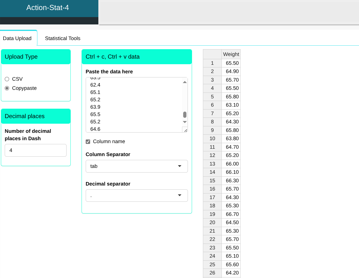
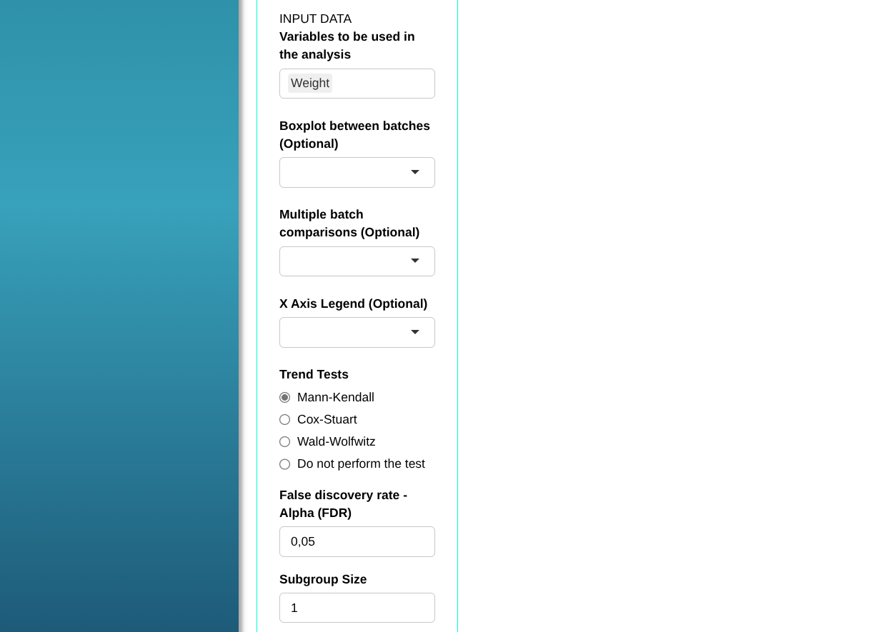
Configuring according to the figure below to perform the analysis.
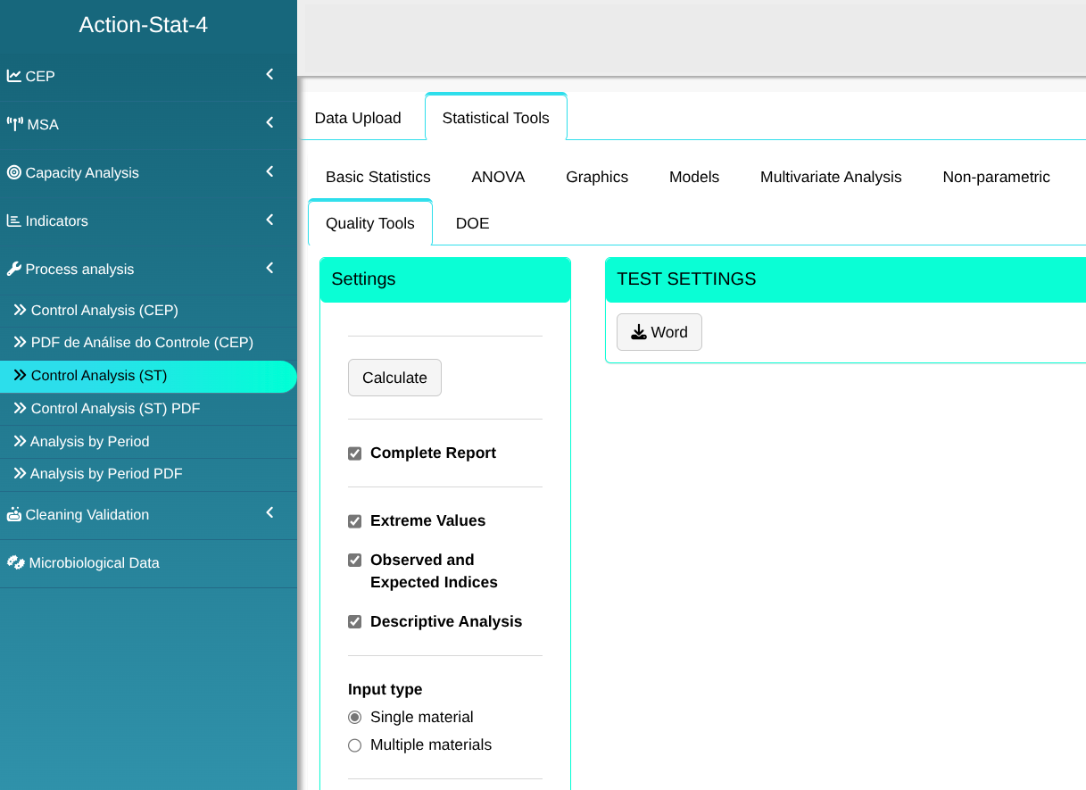

Clicking Calculate displays the results. You can also generate the report and download it as a Word file.
The results are:
Descriptive Summary
|
Statistics |
| Minimum |
60.9 |
| 1º Quartile |
64.425 |
| Mean |
64.9173 |
| Median |
65.1 |
| Tri-Mean |
64.9173 |
| 3º Quartile |
65.575 |
| Maximum |
67.3 |
| Standard Desviation |
1.0953 |
| Coefficient of Variation (%) |
1.6872 |
| Asymetry |
-1.1009 |
| Kurtosis |
2.2197 |
| Range |
6.4 |
| Sample Size |
168 |
Extreme values
|
The order of collection |
Outliers |
| 2 |
98 |
60.9 |
| 3 |
120 |
60.9 |
| 4 |
123 |
60.9 |
| 6 |
152 |
61.6 |
| 7 |
162 |
62.4 |
| 5 |
144 |
62.7 |
| 1 |
61 |
67.3 |
Model linear
|
Model (linear) |
| Intercept |
65.2656 |
| Time |
-0.0041 |
Accuracy Measurement
Process Stability*
Chart of Individual Values and Moving Amplitudes
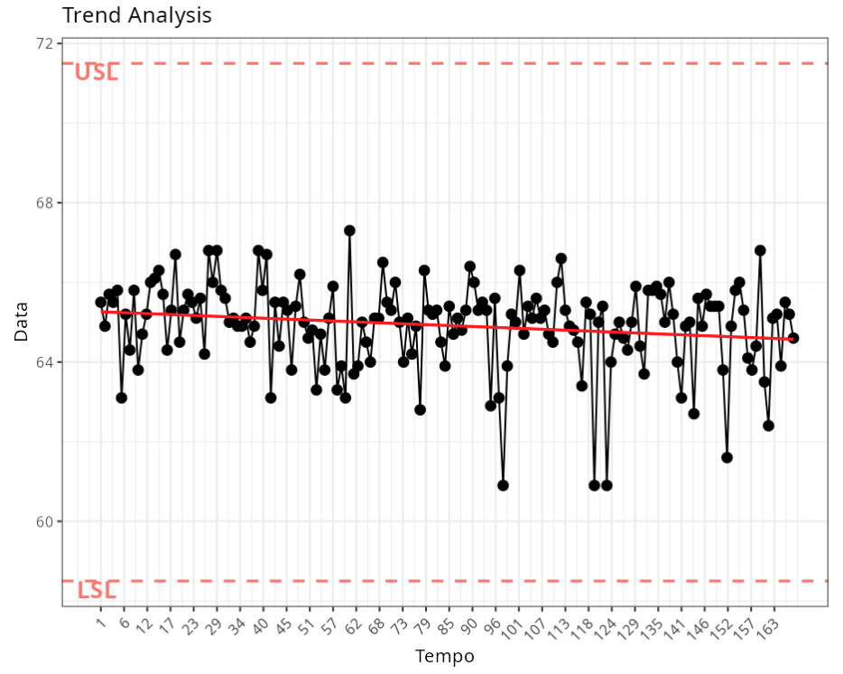
Mann-Kendall
|
Trend Test |
| Statiístic |
-0.106931731104851 |
| P-Value |
0.0428426638245583 |
| Significance Level |
0.05 |
| Conclusion |
Detected Trend |
Automatic Analysis
|
Process Analysis |
Situation |
| 1 |
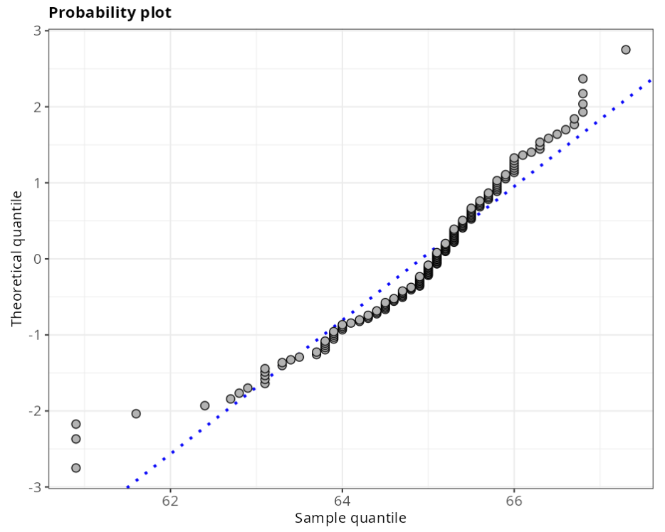
Normality Test |
Normality hypothesis rejected at 5% sifnificance level. |
| 2 |
Box-Cox Transformation |
could not use Box-Cox transformation |
| 3 |
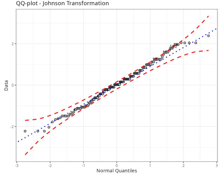
Johnson Transformation |
Data transformation performed with sucess. |
| 4 |
Non-Normal Distribution |
No Aplicable |
| 5 |
Non parametric Distribution |
No Aplicable |
Normality tests
|
Statistics |
P-values |
| Anderson Darling |
2.9789 |
0 |
Estimates
|
Test |
| Gamma |
0.621594044941979 |
| Lambda |
0.82604897976745 |
| Epsilon |
65.538190346758 |
| Eta |
1.17229982993853 |
| Family |
SU |
| P-Value (Anderson-Darling) |
0.5038 |
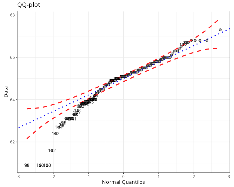
Outliers (Quantiles)
|
obs |
Normal (Quantiles) |
Data |
Criterion |
| 1 |
13 |
1.14 |
1.247 |
Envelope (Confidence Level = 95%) |
| 2 |
15 |
1.44 |
1.589 |
Envelope (Confidence Level = 95%) |
| 3 |
69 |
1.64 |
1.786 |
Envelope (Confidence Level = 95%) |
| 4 |
112 |
1.7 |
1.875 |
Envelope (Confidence Level = 95%) |
| 5 |
19 |
1.77 |
1.96 |
Envelope (Confidence Level = 95%) |
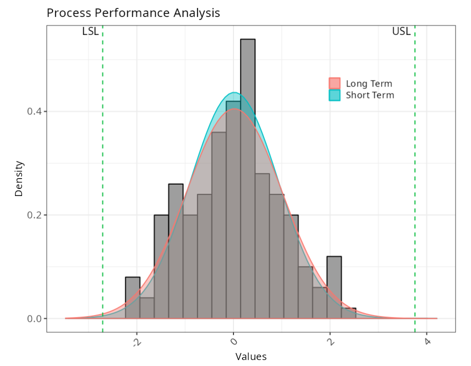
Specifications
|
|
Value |
| 1 |
Sample: |
168 |
| 2 |
Lower Limite |
-2.70659512949514 |
| 3 |
Upper Limite |
3.75677836460632 |
Estimates
|
Value |
| Mean |
0.0184 |
| Standard Desviation (Short term) |
0.9131 |
| Standard Desviation (Long term) |
0.9847 |
|
Performance Indexes ( Total Variability) |
| PP |
1.0940 |
| PPL |
0.9225 |
| PPU |
1.2656 |
| PPK |
0.9225 |
Capacity Indexes (Short term)
|
Capacity Indexes (inherent Variability) |
| CP |
1.1797 |
| CPI |
0.9948 |
| CPS |
1.3647 |
| CPK |
0.9948 |
Observed Indices
|
Observed Indices |
| PPM < LSL |
0 |
| PPM > USE |
0 |
| PPM Total |
0 |
Expected Indexes (Long term)
|
Expected Indexes (Total Variability) |
| PPM < LSL |
2824.8211 |
| PPM > USL |
73.3311 |
| PPM Total |
2898.1522 |
Expected Indexess (Short term)
|
Expected Indexes (Inherent Variability) |
| PPM < LSL |
1421.3225 |
| PPM > USL |
21.1912 |
| PPM Total |
1442.5137 |
SIGMA LEVEL
|
SIGMA LEVEL |
| Zbench (Long term) |
2.7591 |
| Zbench (Short term) |
2.9797 |
| Zshift |
1.5 |
| Sigma Metrics |
4.2591 |