3. Graph by Attributes
Attribute control charts are used in cases where quality characteristics cannot be expressed in terms of numerical values.
Example 1:
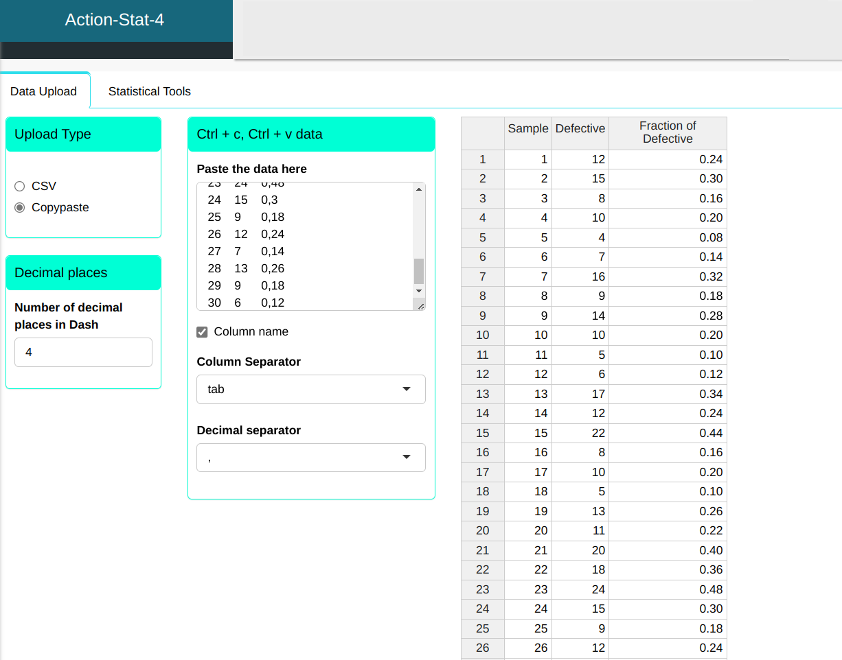
An orange juice factory presented the following data on the number of dented (defective) cans, see table below. In this example, the size of each sample is constant and equal to 50.
| Sample | Defective | Fraction of Defective |
|---|---|---|
| 1 | 12 | 0.24 |
| 2 | 15 | 0.30 |
| 3 | 8 | 0.16 |
| 4 | 10 | 0.20 |
| 5 | 4 | 0.08 |
| 6 | 7 | 0.14 |
| 7 | 16 | 0.32 |
| 8 | 9 | 0.18 |
| 9 | 14 | 0.28 |
| 10 | 10 | 0.20 |
| 11 | 5 | 0.10 |
| 12 | 6 | 0.12 |
| 13 | 17 | 0.34 |
| 14 | 12 | 0.24 |
| 15 | 22 | 0.44 |
| 16 | 8 | 0.16 |
| 17 | 10 | 0.20 |
| 18 | 5 | 0.10 |
| 19 | 13 | 0.26 |
| 20 | 11 | 0.22 |
| 21 | 20 | 0.40 |
| 22 | 18 | 0.36 |
| 23 | 24 | 0.48 |
| 24 | 15 | 0.30 |
| 25 | 9 | 0.18 |
| 26 | 12 | 0.24 |
| 27 | 7 | 0.14 |
| 28 | 13 | 0.26 |
| 29 | 9 | 0.18 |
| 30 | 6 | 0.12 |
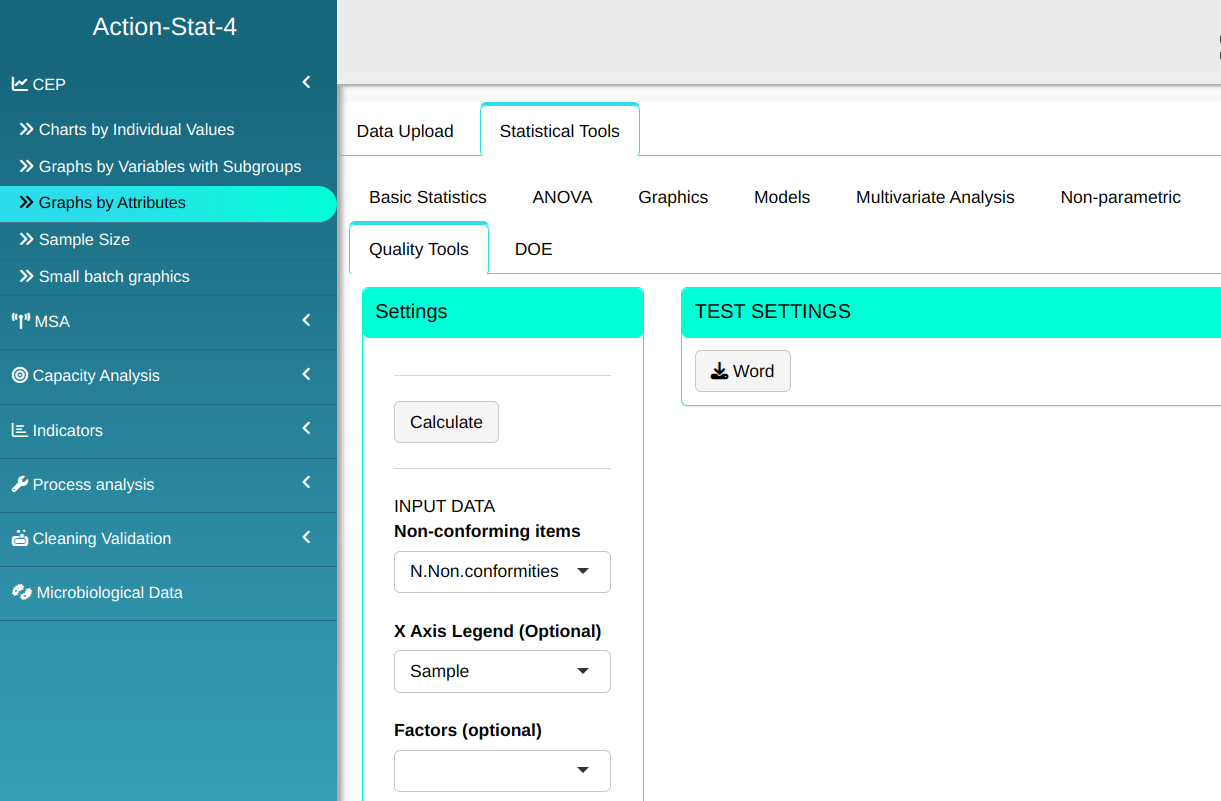
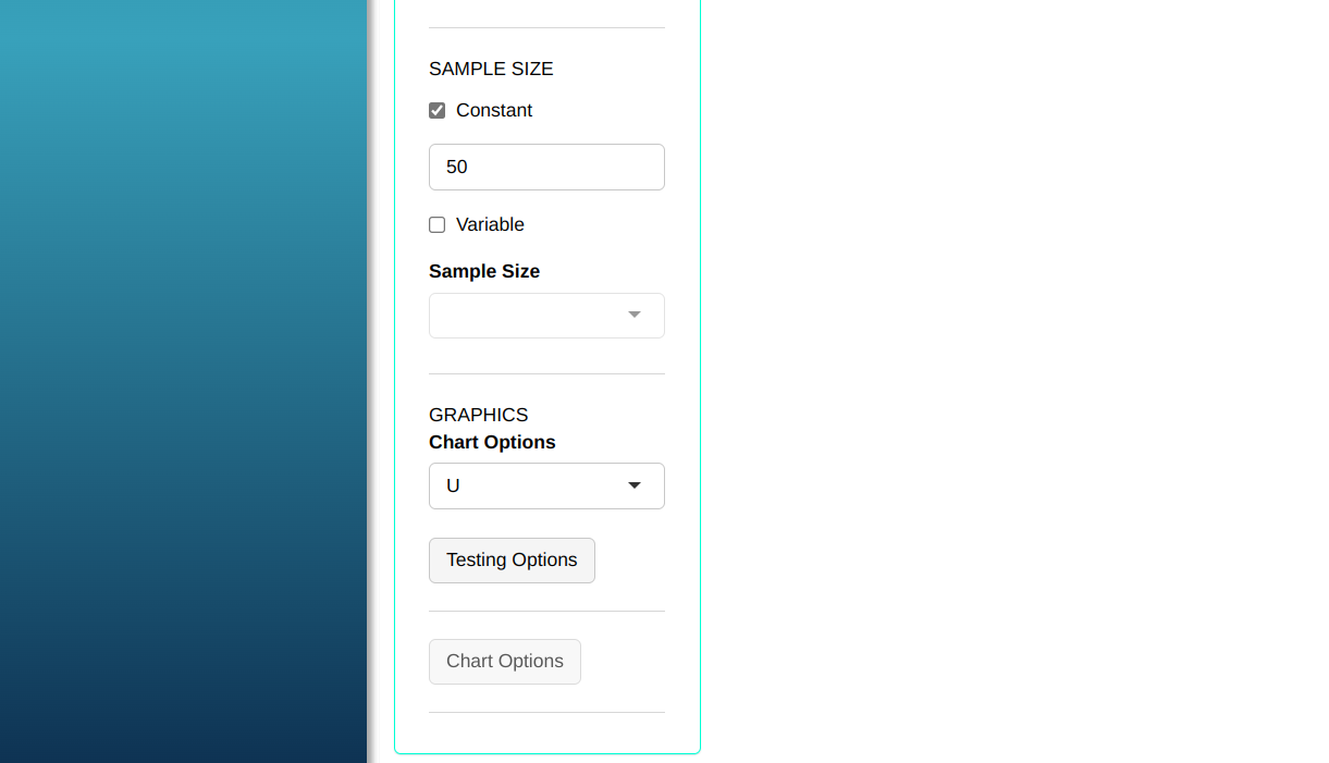
We will upload the data to the system.
Configure as shown in the figure below to perform the graphical analysis.
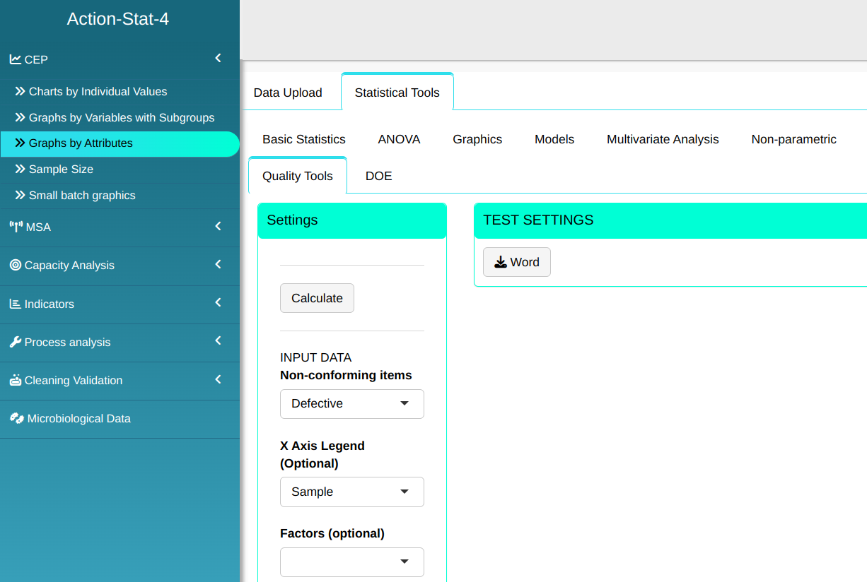
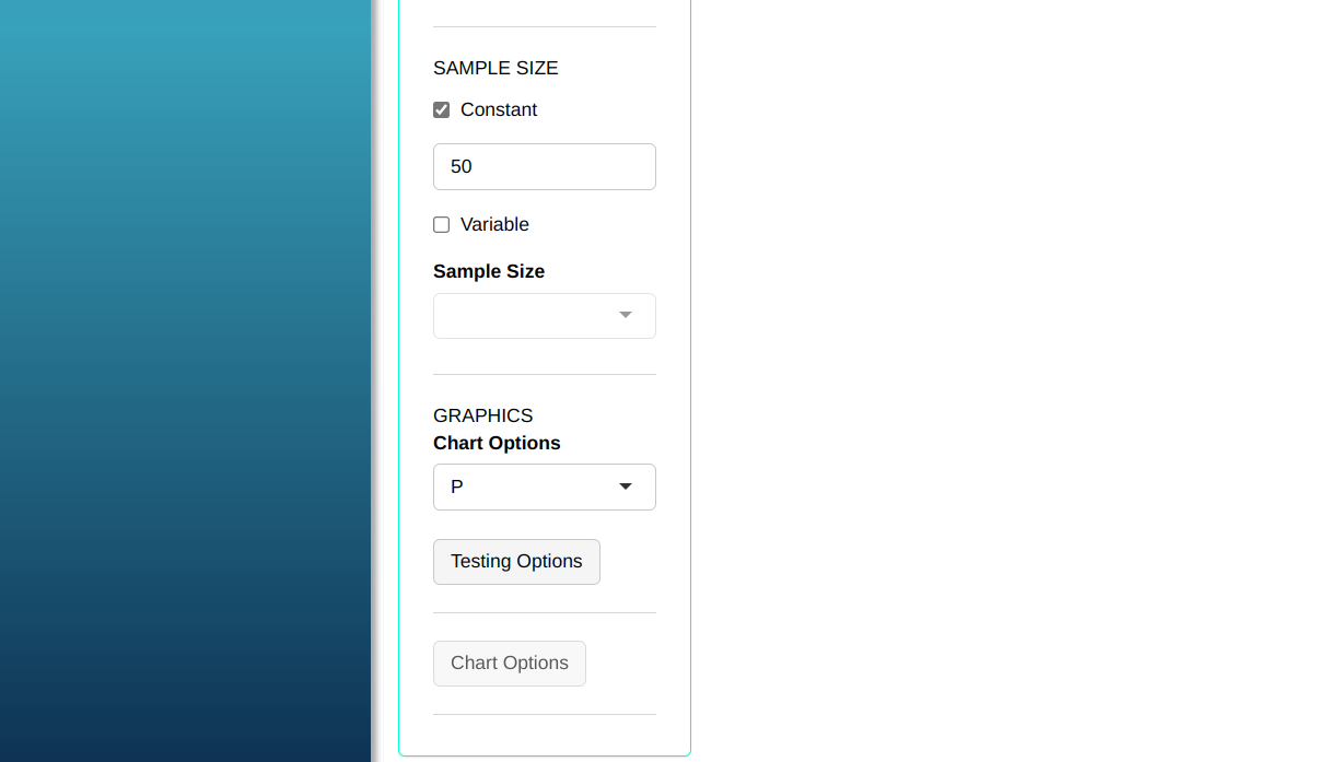
- Click “Test Options” to select the tests you want to run. For some of these tests, you can change the number of points; the software defaults to 1, 9, 6, and 14 points, respectively. For this example, we’ll run all the tests, leaving the software’s default points, and click OK.
Then click Calculate we obtain the results. You can also generate the analyses and download them in Word format.
The results are
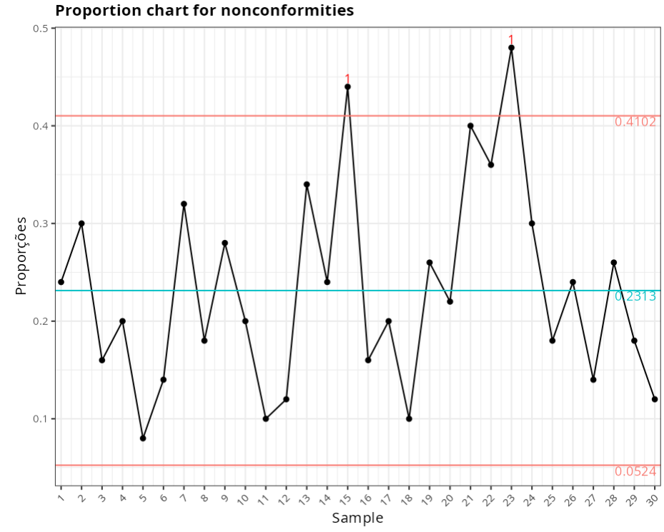
Proportion chart for nonconformities
| Center line | Lower Limit: | Upper Limit: | Fraction Nonconforming |
|---|---|---|---|
| 0.231 | 0.052 | 0.41 | 0.24 |
| 0.231 | 0.052 | 0.41 | 0.3 |
| 0.231 | 0.052 | 0.41 | 0.16 |
| 0.231 | 0.052 | 0.41 | 0.2 |
| 0.231 | 0.052 | 0.41 | 0.08 |
| 0.231 | 0.052 | 0.41 | 0.14 |
| 0.231 | 0.052 | 0.41 | 0.32 |
| 0.231 | 0.052 | 0.41 | 0.18 |
| 0.231 | 0.052 | 0.41 | 0.28 |
| 0.231 | 0.052 | 0.41 | 0.2 |
| 0.231 | 0.052 | 0.41 | 0.1 |
| 0.231 | 0.052 | 0.41 | 0.12 |
| 0.231 | 0.052 | 0.41 | 0.34 |
| 0.231 | 0.052 | 0.41 | 0.24 |
| 0.231 | 0.052 | 0.41 | 0.44 |
| 0.231 | 0.052 | 0.41 | 0.16 |
| 0.231 | 0.052 | 0.41 | 0.2 |
| 0.231 | 0.052 | 0.41 | 0.1 |
| 0.231 | 0.052 | 0.41 | 0.26 |
| 0.231 | 0.052 | 0.41 | 0.22 |
| 0.231 | 0.052 | 0.41 | 0.4 |
| 0.231 | 0.052 | 0.41 | 0.36 |
| 0.231 | 0.052 | 0.41 | 0.48 |
| 0.231 | 0.052 | 0.41 | 0.3 |
| 0.231 | 0.052 | 0.41 | 0.18 |
| 0.231 | 0.052 | 0.41 | 0.24 |
| 0.231 | 0.052 | 0.41 | 0.14 |
| 0.231 | 0.052 | 0.41 | 0.26 |
| 0.231 | 0.052 | 0.41 | 0.18 |
| 0.231 | 0.052 | 0.41 | 0.12 |
Out-of-Control points
| Subgroup | Value | Test |
|---|---|---|
| 15 | 0.44 | 1 point greater than 3 Sigmas from the center line |
| 23 | 0.48 | 1 point greater than 3 Sigmas from the center line |
Example 2:
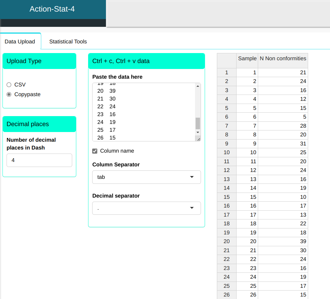
The table shows the number of non-conformities observed in 26 successive samples of 100 printed circuits. Note that for convenience the number of possible non-conformities has been limited to 100, so we have 26 samples with 516 non-conformities.
| Sample | Non conformities |
|---|---|
| 1 | 21 |
| 2 | 24 |
| 3 | 16 |
| 4 | 12 |
| 5 | 15 |
| 6 | 5 |
| 7 | 28 |
| 8 | 20 |
| 9 | 31 |
| 10 | 25 |
| 11 | 20 |
| 12 | 24 |
| 13 | 16 |
| 14 | 19 |
| 15 | 10 |
| 16 | 17 |
| 17 | 13 |
| 18 | 22 |
| 19 | 18 |
| 20 | 39 |
| 21 | 30 |
| 22 | 24 |
| 23 | 16 |
| 24 | 19 |
| 25 | 17 |
| 26 | 15 |
We will upload the data to the system.
Configure as shown in the figure below to perform the graphical analysis.
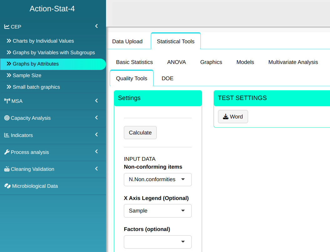
- Click “Test Options” to select the tests you want to run. For some of these tests, you can change the number of points; the software defaults to 1, 9, 6, and 14 points, respectively. For this example, we’ll run all the tests, leaving the software’s default points, and click OK.
Then click Calculate we obtain the results. You can also generate the analyses and download them in Word format.
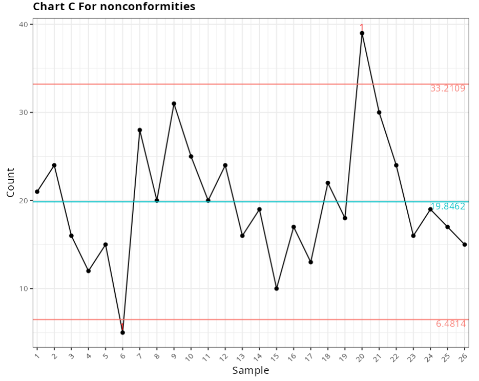
The results are
Chart C for nonconformities
| Center line | Lower Limit: | Upper Limit: | Fraction Nonconforming |
|---|---|---|---|
| 19.846 | 6.481 | 33.2109 | 0.42 |
| 19.846 | 6.481 | 33.2109 | 0.48 |
| 19.846 | 6.481 | 33.2109 | 0.32 |
| 19.846 | 6.481 | 33.2109 | 0.24 |
| 19.846 | 6.481 | 33.2109 | 0.3 |
| 19.846 | 6.481 | 33.2109 | 0.1 |
| 19.846 | 6.481 | 33.2109 | 0.56 |
| 19.846 | 6.481 | 33.2109 | 0.4 |
| 19.846 | 6.481 | 33.2109 | 0.62 |
| 19.846 | 6.481 | 33.2109 | 0.5 |
| 19.846 | 6.481 | 33.2109 | 0.4 |
| 19.846 | 6.481 | 33.2109 | 0.48 |
| 19.846 | 6.481 | 33.2109 | 0.32 |
| 19.846 | 6.481 | 33.2109 | 0.38 |
| 19.846 | 6.481 | 33.2109 | 0.2 |
| 19.846 | 6.481 | 33.2109 | 0.34 |
| 19.846 | 6.481 | 33.2109 | 0.26 |
| 19.846 | 6.481 | 33.2109 | 0.44 |
| 19.846 | 6.481 | 33.2109 | 0.36 |
| 19.846 | 6.481 | 33.2109 | 0.78 |
| 19.846 | 6.481 | 33.2109 | 0.6 |
| 19.846 | 6.481 | 33.2109 | 0.48 |
| 19.846 | 6.481 | 33.2109 | 0.32 |
| 19.846 | 6.481 | 33.2109 | 0.38 |
| 19.846 | 6.481 | 33.2109 | 0.34 |
| 19.846 | 6.481 | 33.2109 | 0.3 |
Out-of-control points
| Subgroup | Value | Test |
|---|---|---|
| 6 | 5 | 1 point greater than 3 Sigmas from the center line |
| 20 | 39 | 1 point greater than 3 Sigmas from the center line |
Example 3:
An orange juice factory presented the following data on the number of crumpled (defective) cans. see table below. In this example, all the samples have constant sizes equal to 50.
| Sample | Defective | Defective Fraction |
|---|---|---|
| 1 | 12 | 0.24 |
| 2 | 15 | 0.30 |
| 3 | 8 | 0.16 |
| 4 | 10 | 0.20 |
| 5 | 4 | 0.08 |
| 6 | 7 | 0.14 |
| 7 | 16 | 0.32 |
| 8 | 9 | 0.18 |
| 9 | 14 | 0.28 |
| 10 | 10 | 0.20 |
| 11 | 5 | 0.10 |
| 12 | 6 | 0.12 |
| 13 | 17 | 0.34 |
| 14 | 12 | 0.24 |
| 15 | 22 | 0.44 |
| 16 | 8 | 0.16 |
| 17 | 10 | 0.20 |
| 18 | 5 | 0.10 |
| 19 | 13 | 0.26 |
| 20 | 11 | 0.22 |
| 21 | 20 | 0.40 |
| 22 | 18 | 0.36 |
| 23 | 24 | 0.48 |
| 24 | 15 | 0.30 |
| 25 | 9 | 0.18 |
| 26 | 12 | 0.24 |
| 27 | 7 | 0.14 |
| 28 | 13 | 0.26 |
| 29 | 9 | 0.18 |
| 30 | 6 | 0.12 |
We will upload the data to the system.
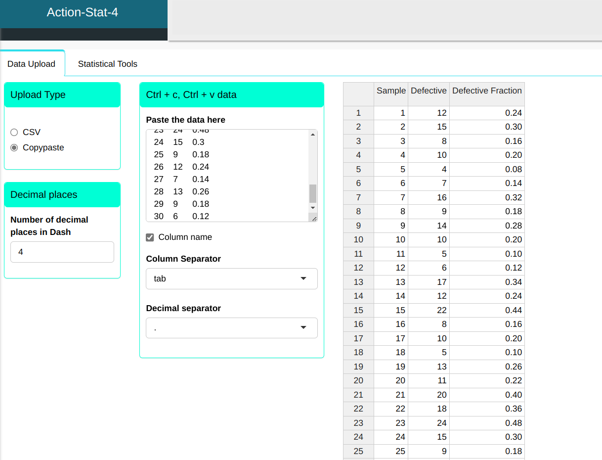
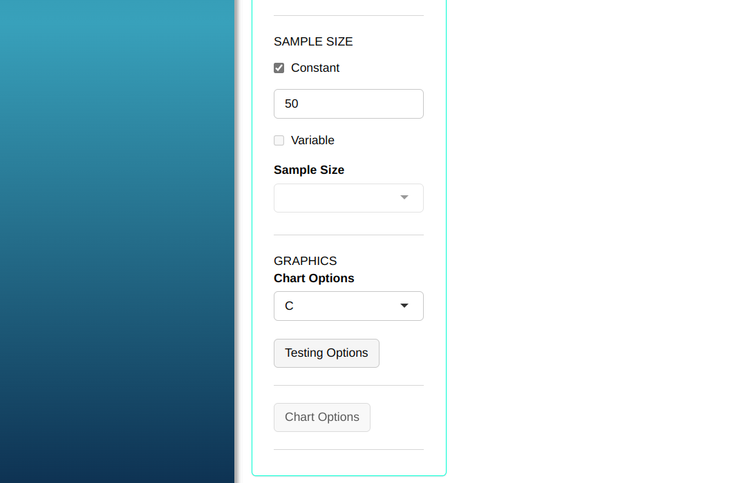
Configure as shown in the figure below to perform the graphical analysis.

- Click “Test Options” to select the tests you want to run. For some of these tests, you can change the number of points; the software defaults to 1, 9, 6, and 14 points, respectively. For this example, we’ll run all the tests, leaving the software’s default points, and click OK.
Then click Calculate we obtain the results. You can also generate the analyses and download them in Word format.
The results are
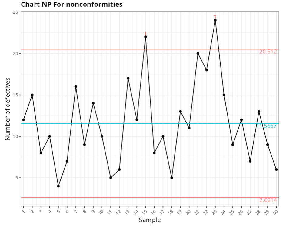
Chart NP For nonconformities
| Center line | Lower Limit | Upper Limit | Fraction Nonconforming |
|---|---|---|---|
| 11.567 | 2.621 | 20.512 | 0.24 |
| 11.567 | 2.621 | 20.512 | 0.3 |
| 11.567 | 2.621 | 20.512 | 0.16 |
| 11.567 | 2.621 | 20.512 | 0.2 |
| 11.567 | 2.621 | 20.512 | 0.08 |
| 11.567 | 2.621 | 20.512 | 0.14 |
| 11.567 | 2.621 | 20.512 | 0.32 |
| 11.567 | 2.621 | 20.512 | 0.18 |
| 11.567 | 2.621 | 20.512 | 0.28 |
| 11.567 | 2.621 | 20.512 | 0.2 |
| 11.567 | 2.621 | 20.512 | 0.1 |
| 11.567 | 2.621 | 20.512 | 0.12 |
| 11.567 | 2.621 | 20.512 | 0.34 |
| 11.567 | 2.621 | 20.512 | 0.24 |
| 11.567 | 2.621 | 20.512 | 0.44 |
| 11.567 | 2.621 | 20.512 | 0.16 |
| 11.567 | 2.621 | 20.512 | 0.2 |
| 11.567 | 2.621 | 20.512 | 0.1 |
| 11.567 | 2.621 | 20.512 | 0.26 |
| 11.567 | 2.621 | 20.512 | 0.22 |
| 11.567 | 2.621 | 20.512 | 0.4 |
| 11.567 | 2.621 | 20.512 | 0.36 |
| 11.567 | 2.621 | 20.512 | 0.48 |
| 11.567 | 2.621 | 20.512 | 0.3 |
| 11.567 | 2.621 | 20.512 | 0.18 |
| 11.567 | 2.621 | 20.512 | 0.24 |
| 11.567 | 2.621 | 20.512 | 0.14 |
| 11.567 | 2.621 | 20.512 | 0.26 |
| 11.567 | 2.621 | 20.512 | 0.18 |
| 11.567 | 2.621 | 20.512 | 0.12 |
Out-of-control points
| Subgroup | Value | Test |
|---|---|---|
| 15 | 22 | 1 point greater than 3 Sigmas from the center line |
| 23 | 24 | 1 point greater than 3 Sigmas from the center line |
Example 4:
Let us consider in the table the number of non-conformities observed in 26 successive samples of 100 printed circuits.Note that for convenience the number of possible non-conformities was limited to 100, so we have 26 samples with 516 non-conformities. (Table of example 2)
| Sample | Non conformities |
|---|---|
| 1 | 21 |
| 2 | 24 |
| 3 | 16 |
| 4 | 12 |
| 5 | 15 |
| 6 | 5 |
| 7 | 28 |
| 8 | 20 |
| 9 | 31 |
| 10 | 25 |
| 11 | 20 |
| 12 | 24 |
| 13 | 16 |
| 14 | 19 |
| 15 | 10 |
| 16 | 17 |
| 17 | 13 |
| 18 | 22 |
| 19 | 18 |
| 20 | 39 |
| 21 | 30 |
| 22 | 24 |
| 23 | 16 |
| 24 | 19 |
| 25 | 17 |
| 26 | 15 |
We will upload the data to the system.
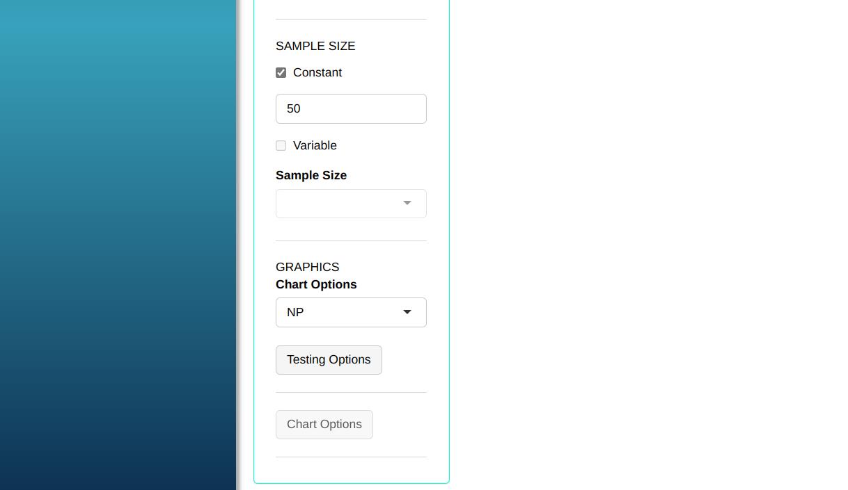
Configure as shown in the figure below to perform the graphical analysis.
- Click “Test Options” to select the tests you want to run. For some of these tests, you can change the number of points; the software defaults to 1, 9, 6, and 14 points, respectively. For this example, we’ll run all the tests, leaving the software’s default points, and click OK.
Then click Calculate we obtain the results. You can also generate the analyses and download them in Word format.
The results are
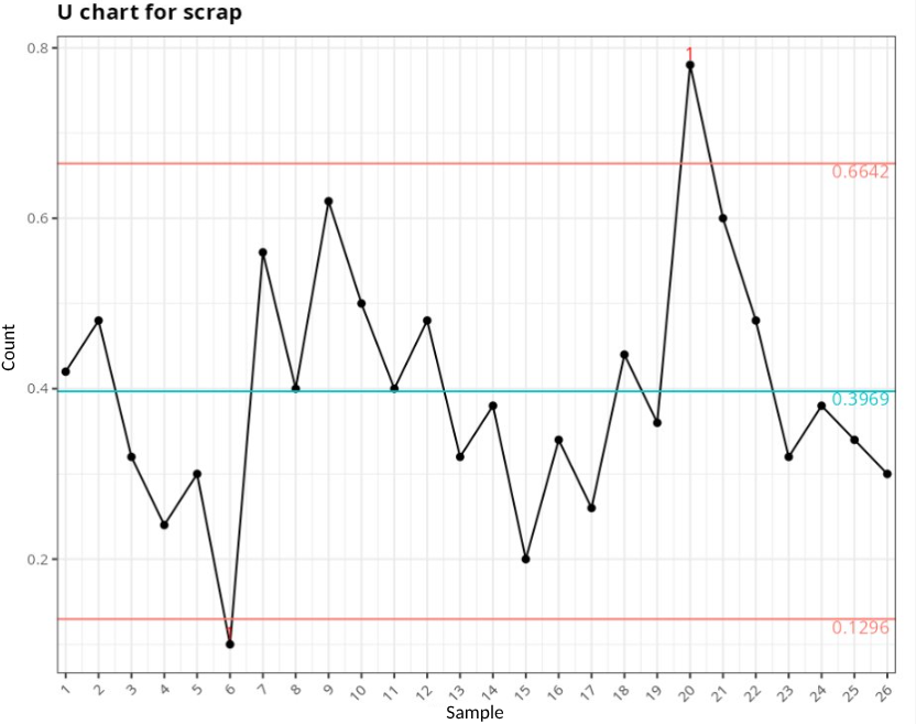
Proportion chart for nonconformities
| Center Line | Lower Limit | Upper Limit | Fraction Nonconforming |
|---|---|---|---|
| 0.397 | 0.13 | 0.664 | 0.42 |
| 0.397 | 0.13 | 0.664 | 0.48 |
| 0.397 | 0.13 | 0.664 | 0.32 |
| 0.397 | 0.13 | 0.664 | 0.24 |
| 0.397 | 0.13 | 0.664 | 0.3 |
| 0.397 | 0.13 | 0.664 | 0.1 |
| 0.397 | 0.13 | 0.664 | 0.56 |
| 0.397 | 0.13 | 0.664 | 0.4 |
| 0.397 | 0.13 | 0.664 | 0.62 |
| 0.397 | 0.13 | 0.664 | 0.5 |
| 0.397 | 0.13 | 0.664 | 0.4 |
| 0.397 | 0.13 | 0.664 | 0.48 |
| 0.397 | 0.13 | 0.664 | 0.32 |
| 0.397 | 0.13 | 0.664 | 0.38 |
| 0.397 | 0.13 | 0.664 | 0.2 |
| 0.397 | 0.13 | 0.664 | 0.34 |
| 0.397 | 0.13 | 0.664 | 0.26 |
| 0.397 | 0.13 | 0.664 | 0.44 |
| 0.397 | 0.13 | 0.664 | 0.36 |
| 0.397 | 0.13 | 0.664 | 0.78 |
| 0.397 | 0.13 | 0.664 | 0.6 |
| 0.397 | 0.13 | 0.664 | 0.48 |
| 0.397 | 0.13 | 0.664 | 0.32 |
| 0.397 | 0.13 | 0.664 | 0.38 |
| 0.397 | 0.13 | 0.664 | 0.34 |
| 0.397 | 0.13 | 0.664 | 0.3 |
Out-of-control points
| Subgroup | Value | Test |
|---|---|---|
| 6 | 0.10 | 1 point greater than 3 Sigmas from the center line |
| 20 | 0.78 | 1 point greater than 3 Sigmas from the center line |
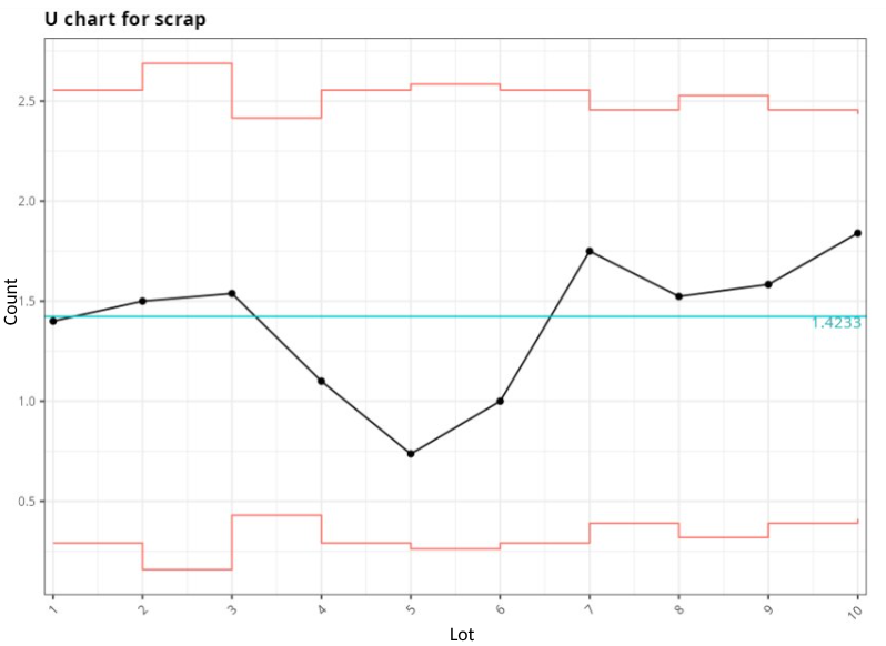
Example 5:
In a textile company the dyed garments are inspected for defects over 50 square meters. The data for the 10 inspection lots is shown in the table.
| Lot | Qty. square meters | Non-conformity | Units inspected |
|---|---|---|---|
| 1 | 500 | 14 | 10 |
| 2 | 400 | 12 | 8 |
| 3 | 650 | 20 | 13 |
| 4 | 500 | 11 | 10 |
| 5 | 475 | 7 | 9.5 |
| 6 | 500 | 10 | 10 |
| 7 | 600 | 21 | 12 |
| 8 | 525 | 16 | 10.5 |
| 9 | 600 | 19 | 12 |
| 10 | 625 | 23 | 12.5 |
We will upload the data to the system.
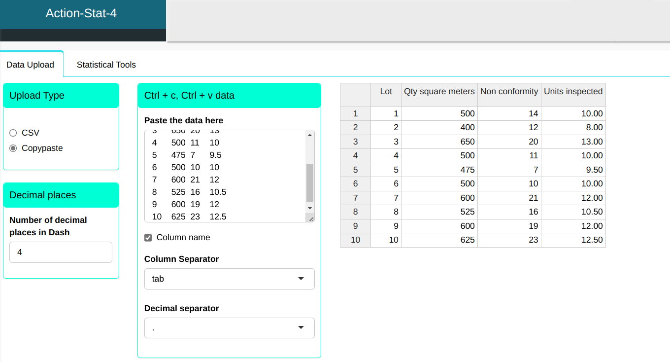
Configure as shown in the figure below to perform the graphical analysis.
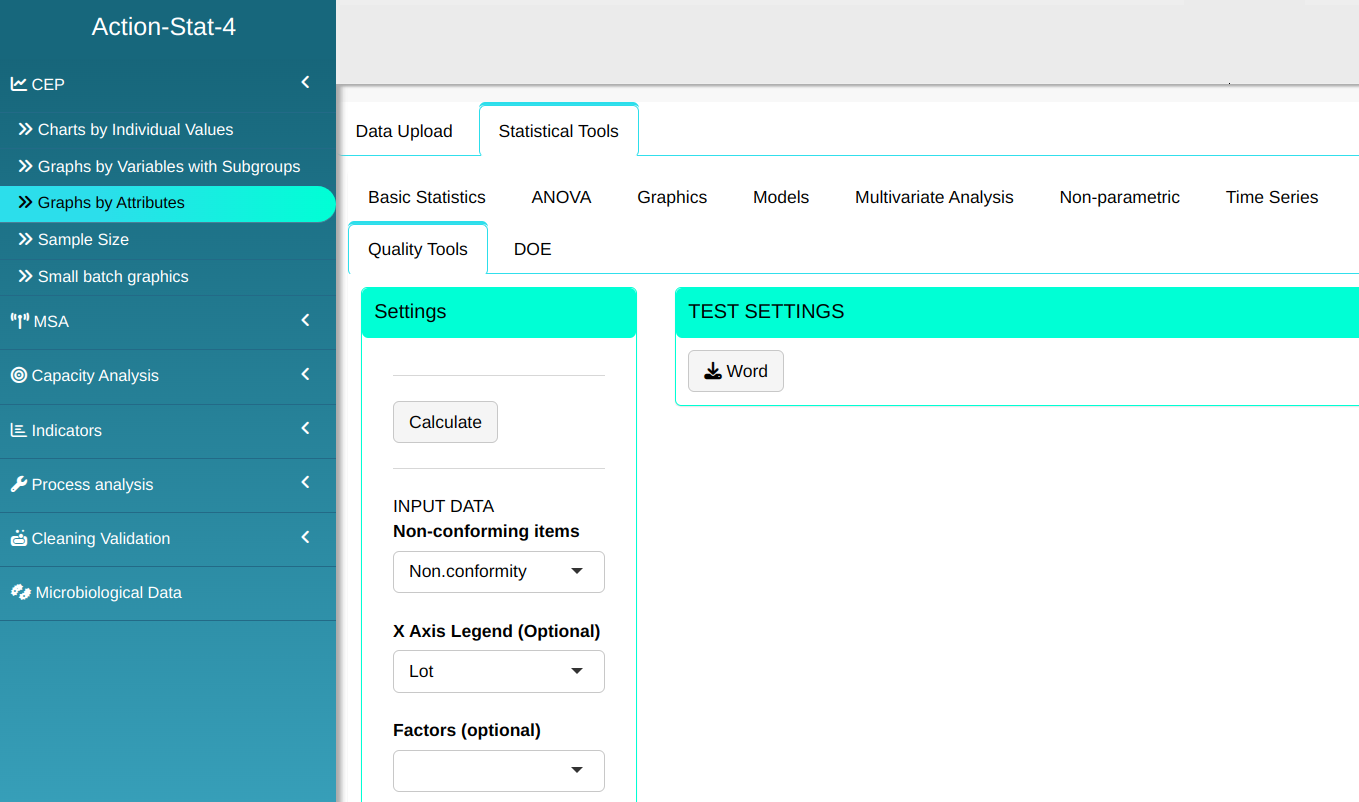
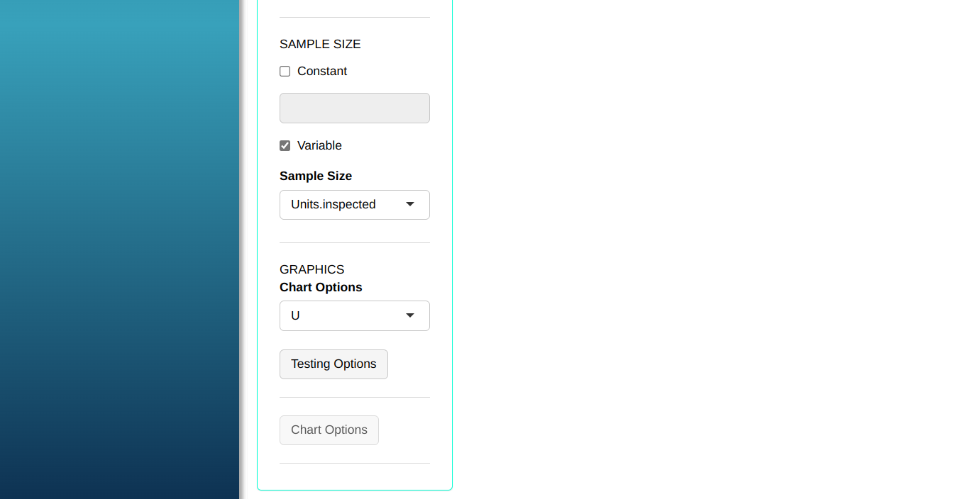
- Click “Test Options” to select the tests you want to run. For some of these tests, you can change the number of points; the software defaults to 1, 9, 6, and 14 points, respectively. For this example, we’ll run all the tests, leaving the software’s default points, and click OK.
Then click Calculate we obtain the results. You can also generate the analyses and download them in Word format.
The results are:
Proportion chart for nonconformities
| Center Line | Lower Limit | Upper Limit | Fraction Nonconforming |
|---|---|---|---|
| 1.423 | 0.291 | 2.555 | 1.400 |
| 1.423 | 0.158 | 2.689 | 1.500 |
| 1.423 | 0.431 | 2.416 | 1.538 |
| 1.423 | 0.291 | 2.555 | 1.100 |
| 1.423 | 0.262 | 2.584 | 0.737 |
| 1.423 | 0.291 | 2.555 | 1.000 |
| 1.423 | 0.390 | 2.456 | 1.750 |
| 1.423 | 0.319 | 2.528 | 1.524 |
| 1.423 | 0.390 | 2.456 | 1.583 |
| 1.423 | 0.411 | 2.436 | 1.840 |