5. Graphics for Small Lots
To attaining process efficiencies for small lots. it is essential that SPC methods can verify that the process is truly under statistical control. i.e. that it is predictable and can detect variations due to special causes during these small “lots”.
Example 1:
In the rough machining of external diameters (shafts) on a lathe. 25 samples were taken. each consisting of 3 pieces. obtaining the values in the table below.
| Sample | N | Pieces | P1 | P2 | P3 |
|---|---|---|---|---|---|
| 1 | 220 | 1 | 219.7838 | 220.0287 | 220.0922 |
| 2 | 220 | 1 | 219.9046 | 220.1229 | 220.2368 |
| 3 | 220 | 1 | 219.8345 | 220.0862 | 219.9268 |
| 4 | 220 | 1 | 219.7302 | 220.001 | 220.0357 |
| 5 | 220 | 1 | 220.1644 | 220.3151 | 219.9806 |
| 6 | 260 | 2 | 259.8635 | 260.1847 | 259.867 |
| 7 | 260 | 2 | 259.7917 | 259.9042 | 259.908 |
| 8 | 260 | 2 | 259.8264 | 259.8535 | 259.6465 |
| 9 | 260 | 2 | 259.6421 | 260.0869 | 259.9488 |
| 10 | 260 | 2 | 259.8945 | 260.0154 | 260.3685 |
| 11 | 320 | 3 | 319.7366 | 319.5236 | 319.7053 |
| 12 | 320 | 3 | 319.8834 | 319.415 | 319.8163 |
| 13 | 320 | 3 | 320.2431 | 320.1935 | 319.9893 |
| 14 | 320 | 3 | 319.9805 | 320.0828 | 320.0418 |
| 15 | 320 | 3 | 320.4944 | 320.4552 | 320.0477 |
| 16 | 240 | 4 | 239.8076 | 239.7787 | 240.2064 |
| 17 | 240 | 4 | 240.1663 | 240.1888 | 240.2023 |
| 18 | 240 | 4 | 240.1662 | 240.1382 | 240.1141 |
| 19 | 240 | 4 | 240.017 | 239.9212 | 240.0397 |
| 20 | 240 | 4 | 240.2081 | 240.0484 | 239.9119 |
| 21 | 300 | 5 | 300.0479 | 300.1325 | 299.9955 |
| 22 | 300 | 5 | 300.2815 | 299.9451 | 300.0365 |
| 23 | 300 | 5 | 299.7173 | 300.383 | 300.4608 |
| 24 | 300 | 5 | 300.0009 | 300.0487 | 300.0038 |
| 25 | 300 | 5 | 299.5822 | 300.4351 | 299.7919 |
We will upload the data to the system.
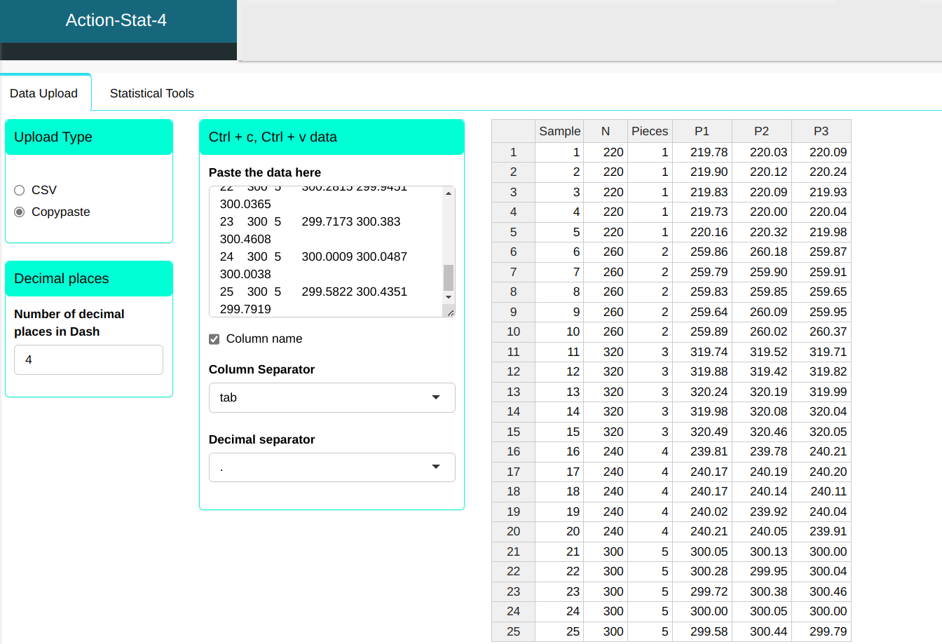
Configure as shown in the figure below to perform the graphical analysis.
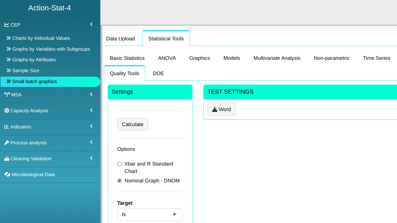

Then click Calculate we obtain the results. You can also generate the analyses and download them in Word format.

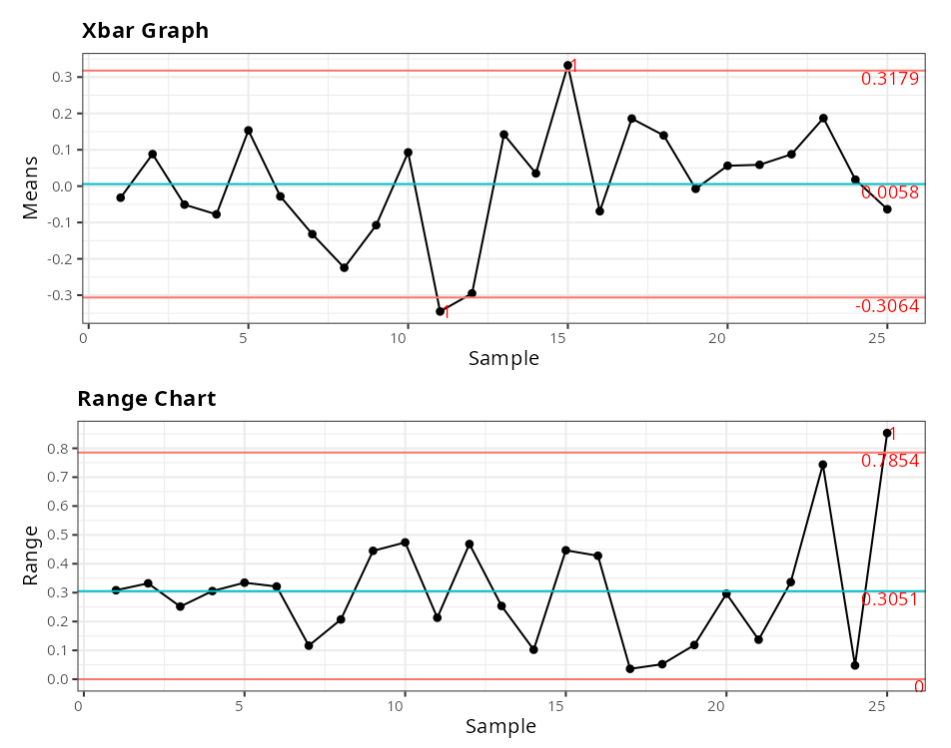
The results are:
Limits - Xbar
| Limits | |
|---|---|
| Upper Limit | 0.318 |
| Center line | 0.006 |
| Lower Limit | -0.306 |
Limits - R
| Limits | |
|---|---|
| Standard Deviation | 0.180 |
| Upper Limit | 0.785 |
| Center line | 0.305 |
| Lower Limit | 0.000 |
Example 2:
In the rough machining of external diameters (shafts) on a lathe. 25 samples were taken. each consisting of 3 pieces. obtaining the values in the table below.
| Sample | N | Piece | P1 | P2 | P3 |
|---|---|---|---|---|---|
| 1 | 220 | 1 | 219.7838 | 220.0287 | 220.0922 |
| 2 | 220 | 1 | 219.9046 | 220.1229 | 220.2368 |
| 3 | 220 | 1 | 219.8345 | 220.0862 | 219.9268 |
| 4 | 220 | 1 | 219.7302 | 220.001 | 220.0357 |
| 5 | 220 | 1 | 220.1644 | 220.3151 | 219.9806 |
| 6 | 260 | 2 | 259.8635 | 260.1847 | 259.867 |
| 7 | 260 | 2 | 259.7917 | 259.9042 | 259.908 |
| 8 | 260 | 2 | 259.8264 | 259.8535 | 259.6465 |
| 9 | 260 | 2 | 259.6421 | 260.0869 | 259.9488 |
| 10 | 260 | 2 | 259.8945 | 260.0154 | 260.3685 |
| 11 | 320 | 3 | 319.7366 | 319.5236 | 319.7053 |
| 12 | 320 | 3 | 319.8834 | 319.415 | 319.8163 |
| 13 | 320 | 3 | 320.2431 | 320.1935 | 319.9893 |
| 14 | 320 | 3 | 319.9805 | 320.0828 | 320.0418 |
| 15 | 320 | 3 | 320.4944 | 320.4552 | 320.0477 |
| 16 | 240 | 4 | 239.8076 | 239.7787 | 240.2064 |
| 17 | 240 | 4 | 240.1663 | 240.1888 | 240.2023 |
| 18 | 240 | 4 | 240.1662 | 240.1382 | 240.1141 |
| 19 | 240 | 4 | 240.017 | 239.9212 | 240.0397 |
| 20 | 240 | 4 | 240.2081 | 240.0484 | 239.9119 |
| 21 | 300 | 5 | 300.0479 | 300.1325 | 299.9955 |
| 22 | 300 | 5 | 300.2815 | 299.9451 | 300.0365 |
| 23 | 300 | 5 | 299.7173 | 300.383 | 300.4608 |
| 24 | 300 | 5 | 300.0009 | 300.0487 | 300.0038 |
| 25 | 300 | 5 | 299.5822 | 300.4351 | 299.7919 |
We will upload the data to the system.
Configure as shown in the figure below to perform the graphical analysis.


Then click Calculate we obtain the results. You can also generate the analyses and download them in Word format.
The results are:
Estimates by part
| Parts | Standardized mean | Standardized Range | Estimates of standard deviation |
|---|---|---|---|
| 1 | 220.016 | 0.306 | 0.181 |
| 2 | 259.920 | 0.313 | 0.185 |
| 3 | 319.974 | 0.297 | 0.175 |
| 4 | 240.061 | 0.186 | 0.110 |
| 5 | 300.058 | 0.424 | 0.250 |
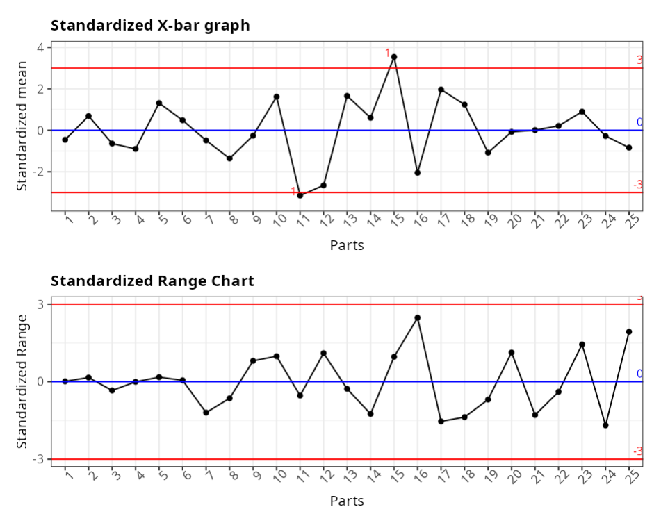
Standardization by sample
| Parts | Standardized Mean | Standardized Range | |
|---|---|---|---|
| 1 | 1 | -0.459 | 0.012 |
| 2 | 1 | 0.687 | 0.16 |
| 3 | 1 | -0.642 | -0.341 |
| 4 | 1 | -0.899 | -0.006 |
| 5 | 1 | 1.312 | 0.174 |
| 6 | 2 | 0.484 | 0.052 |
| 7 | 2 | -0.489 | -1.197 |
| 8 | 2 | -1.356 | -0.644 |
| 9 | 2 | -0.258 | 0.806 |
| 10 | 2 | 1.619 | 0.984 |
| 11 | 3 | -3.148 | -0.538 |
| 12 | 3 | -2.657 | 1.102 |
| 13 | 3 | 1.66 | -0.276 |
| 14 | 3 | 0.604 | -1.249 |
| 15 | 3 | 3.541 | 0.962 |
| 16 | 4 | -2.049 | 2.474 |
| 17 | 4 | 1.966 | -1.537 |
| 18 | 4 | 1.237 | -1.372 |
| 19 | 4 | -1.077 | -0.692 |
| 20 | 4 | -0.077 | 1.128 |
| 21 | 5 | 0.008 | -1.289 |
| 22 | 5 | 0.209 | -0.392 |
| 23 | 5 | 0.897 | 1.44 |
| 24 | 5 | -0.275 | -1.691 |
| 25 | 5 | -0.838 | 1.932 |