4. Trend and Linearity
Linearity is measured by the slope of the line formed by the different reference values in relation to their trend. The less steep the line, the better the quality of the measurement systems.
Example 1:
As an application of a trend and linearity study, we are going to evaluate a measurement system for measuring the temperature of a furnace using an optical pyrometer. To do this, we are going to carry out a study by comparison with a standard element term. We will take 5 temperature levels:
| Standard | Measure | VR | Tolerance |
|---|---|---|---|
| 1 | 748.8 | 750 | 100 |
| 1 | 749.8 | 750 | 100 |
| 1 | 748.8 | 750 | 100 |
| 1 | 748.8 | 750 | 100 |
| 1 | 748.8 | 750 | 100 |
| 1 | 748.8 | 750 | 100 |
| 1 | 747.7 | 750 | 100 |
| 1 | 747.7 | 750 | 100 |
| 1 | 747.7 | 750 | 100 |
| 1 | 748.7 | 750 | 100 |
| 1 | 749.7 | 750 | 100 |
| 1 | 750.7 | 750 | 100 |
| 2 | 848.8 | 850 | 100 |
| 2 | 848.8 | 850 | 100 |
| 2 | 848.8 | 850 | 100 |
| 2 | 847.2 | 850 | 100 |
| 2 | 847.2 | 850 | 100 |
| 2 | 847.2 | 850 | 100 |
| 2 | 846.1 | 850 | 100 |
| 2 | 846.1 | 850 | 100 |
| 2 | 846.2 | 850 | 100 |
| 2 | 846.3 | 850 | 100 |
| 2 | 847.3 | 850 | 100 |
| 2 | 848.3 | 850 | 100 |
| 3 | 946.9 | 950 | 100 |
| 3 | 946.9 | 950 | 100 |
| 3 | 946.9 | 950 | 100 |
| 3 | 945.8 | 950 | 100 |
| 3 | 944.8 | 950 | 100 |
| 3 | 944.8 | 950 | 100 |
| 3 | 943.6 | 950 | 100 |
| 3 | 943.6 | 950 | 100 |
| 3 | 943.6 | 950 | 100 |
| 3 | 945.1 | 950 | 100 |
| 3 | 946.1 | 950 | 100 |
| 3 | 947.1 | 950 | 100 |
| 4 | 1045.4 | 1050 | 100 |
| 4 | 1045.4 | 1050 | 100 |
| 4 | 1045.4 | 1050 | 100 |
| 4 | 1044.9 | 1050 | 100 |
| 4 | 1043.9 | 1050 | 100 |
| 4 | 1044.9 | 1050 | 100 |
| 4 | 1042 | 1050 | 100 |
| 4 | 1042 | 1050 | 100 |
| 4 | 1042 | 1050 | 100 |
| 4 | 1045.6 | 1050 | 100 |
| 4 | 1046.6 | 1050 | 100 |
| 4 | 1047.6 | 1050 | 100 |
| 5 | 1141.9 | 1150 | 100 |
| 5 | 1141.3 | 1150 | 100 |
| 5 | 1142.9 | 1150 | 100 |
| 5 | 1144.3 | 1150 | 100 |
| 5 | 1143.5 | 1150 | 100 |
| 5 | 1140.9 | 1150 | 100 |
| 5 | 1141.9 | 1150 | 100 |
| 5 | 1142.2 | 1150 | 100 |
| 5 | 1142.1 | 1150 | 100 |
| 5 | 1140 | 1150 | 100 |
| 5 | 1140.7 | 1150 | 100 |
| 5 | 1142.7 | 1150 | 100 |
We will upload the data to the system.
Configuring as shown in the figure below to perform the analysis.
Then click Calculate to get the results. You can also generate the analyses and download them in Word format.

The results are:
Analysis result
| LINEARITY ANALYSIS |
Linear Regression Coefficients Test
| Estimate | Stadard Deviation | t Statistic | P-value | |
|---|---|---|---|---|
| (Intercept) | 11.161 | 1.167 | 9.567 | 0 |
| Angular Coefficient | -0.016 | 0.001 | -13.433 | 0 |
Descriptive Measure of Fit Quality
| R^2 | Adjusted R^2 | t Statistic |
|---|---|---|
| 0.757 | 0.753 | 180.456 |
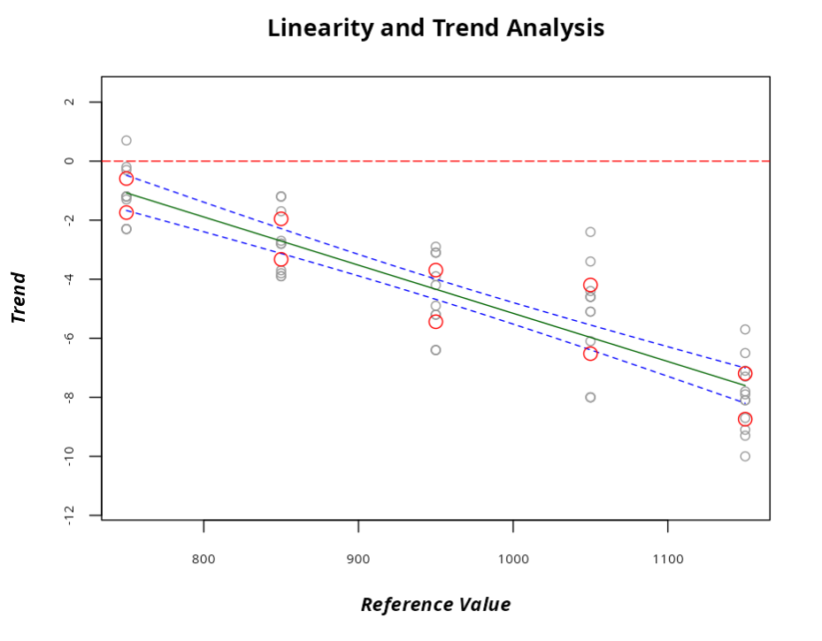
Resultado da análise
| Linearity and Trend Analysis |
TREND ANALYSIS -t-Test
| Reference Value | Mean | Trend | t Statistic | P-value | Lower Limit | Upper Limit | EV % | Standard Deviation |
|---|---|---|---|---|---|---|---|---|
| 750 | 748.833 | -1.167 | -4.456 | 0.001 | -1.743 | -0.590 | 5.441 | 0.907 |
| 850 | 847.358 | -2.642 | -8.474 | 0.000 | -3.328 | -1.956 | 6.480 | 1.080 |
| 950 | 945.433 | -4.567 | -11.502 | 0.000 | -5.441 | -3.693 | 8.252 | 1.375 |
| 1050 | 1044.642 | -5.358 | -10.142 | 0.000 | -6.521 | -4.195 | 10.982 | 1.830 |
| 1150 | 1142.033 | -7.967 | -22.680 | 0.000 | -8.740 | -7.194 | 7.301 | 1.217 |
Resultado da Análise
| Mean of Trend | ||
| $\qquad \quad$-4.34 |
Example 2:
The measurement system engineer was interested in determining the linearity of a measurement system. Five standard pieces, which are distributed the entire variation range of the process, were measured 15 times in the measurement laboratory to determine the reference value. In this case, the metrologist used a measuring instrument with a better resolution than the instrument normally used. After determining the reference value, an evaluator took 12 measurements of each standard piece. The values are summarized in the table below. Here. we have g=5 (number of pieces) and m=12 (readings on each piece).
| Piece | Measurement | VR | History |
|---|---|---|---|
| 1 | 2.7 | 2 | 0.744067 |
| 2 | 2.5 | 2 | 0.744067 |
| 3 | 2.4 | 2 | 0.744067 |
| 4 | 2.5 | 2 | 0.744067 |
| 5 | 2.7 | 2 | 0.744067 |
| 6 | 2.3 | 2 | 0.744067 |
| 7 | 2.5 | 2 | 0.744067 |
| 8 | 2.5 | 2 | 0.744067 |
| 9 | 2.4 | 2 | 0.744067 |
| 10 | 2.4 | 2 | 0.744067 |
| 11 | 2.6 | 2 | 0.744067 |
| 12 | 2.4 | 2 | 0.744067 |
| 1 | 5.1 | 4 | 2.684806 |
| 2 | 3.9 | 4 | 2.684806 |
| 3 | 4.2 | 4 | 2.684806 |
| 4 | 5 | 4 | 2.684806 |
| 5 | 3.8 | 4 | 2.684806 |
| 6 | 3.9 | 4 | 2.684806 |
| 7 | 3.9 | 4 | 2.684806 |
| 8 | 3.9 | 4 | 2.684806 |
| 9 | 3.9 | 4 | 2.684806 |
| 10 | 4 | 4 | 2.684806 |
| 11 | 4.1 | 4 | 2.684806 |
| 12 | 3.8 | 4 | 2.684806 |
| 1 | 5.8 | 6 | 1.175894 |
| 2 | 5.7 | 6 | 1.175894 |
| 3 | 5.9 | 6 | 1.175894 |
| 4 | 5.9 | 6 | 1.175894 |
| 5 | 6 | 6 | 1.175894 |
| 6 | 6.1 | 6 | 1.175894 |
| 7 | 6 | 6 | 1.175894 |
| 8 | 6.1 | 6 | 1.175894 |
| 9 | 6.4 | 6 | 1.175894 |
| 10 | 6.3 | 6 | 1.175894 |
| 11 | 6 | 6 | 1.175894 |
| 12 | 6.1 | 6 | 1.175894 |
| 1 | 7.6 | 8 | 0.597723 |
| 2 | 7.7 | 8 | 0.597723 |
| 3 | 7.8 | 8 | 0.597723 |
| 4 | 7.7 | 8 | 0.597723 |
| 5 | 7.8 | 8 | 0.597723 |
| 6 | 7.8 | 8 | 0.597723 |
| 7 | 7.8 | 8 | 0.597723 |
| 8 | 7.7 | 8 | 0.597723 |
| 9 | 7.8 | 8 | 0.597723 |
| 10 | 7.5 | 8 | 0.597723 |
| 11 | 7.6 | 8 | 0.597723 |
| 12 | 7.7 | 8 | 0.597723 |
| 1 | 9.1 | 10 | 0.880083 |
| 2 | 9.3 | 10 | 0.880083 |
| 3 | 9.5 | 10 | 0.880083 |
| 4 | 9.3 | 10 | 0.880083 |
| 5 | 9.4 | 10 | 0.880083 |
| 6 | 9.5 | 10 | 0.880083 |
| 7 | 9.5 | 10 | 0.880083 |
| 8 | 9.5 | 10 | 0.880083 |
| 9 | 9.6 | 10 | 0.880083 |
| 10 | 9.2 | 10 | 0.880083 |
| 11 | 9.3 | 10 | 0.880083 |
| 12 | 9.4 | 10 | 0.880083 |
We will upload the data to the system.
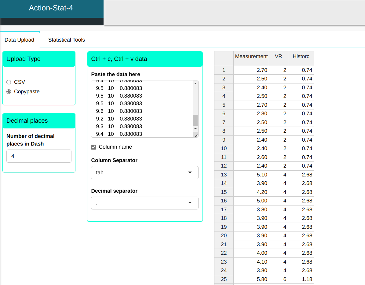
Configuring as shown in the figure below to perform the analysis.
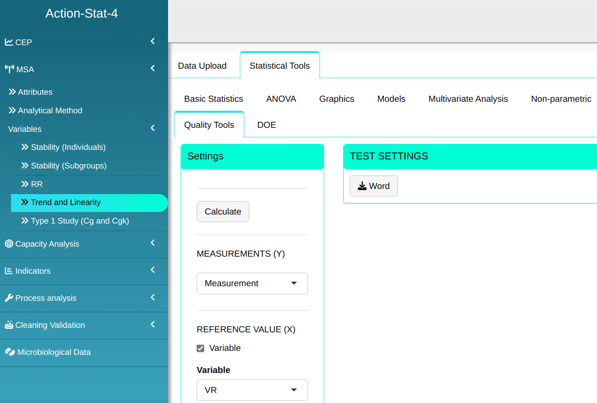
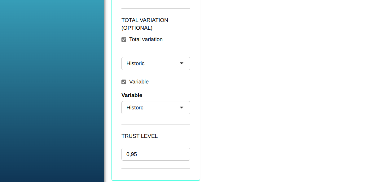
Then click Calculate to get the results. You can also generate the analyses and download them in Word format.
The results are:
Analysis result
| LINEARITY ANALYSIS |
Linear Regression Coefficients Tests
| Estimate | Standard Deviation | t Statistic | P-value | |
|---|---|---|---|---|
| (Intercept) | 0.737 | 0.073 | 10.158 | 0 |
| Angular Coefficient | -0.132 | 0.011 | -12.043 | 0 |
Descriptive Measure of Fit Quality
| R^2 | Adjusted R^2 | t Statistic |
|---|---|---|
| 0.714 | 0.709 | 145.023 |
Resultado da análise
| Linearity and Trend Analysis |
TREND ANALYSIS -t-Test
| Refference Valur | Mean | Trend | t Statistic | P-value | Lower Limit | Upper Limit | VE % | Standard Deviation |
|---|---|---|---|---|---|---|---|---|
| 2 | 2.492 | 0.492 | 13.734 | 0 | 0.413 | 0.57 | 16.666 | 0.124 |
| 4 | 4.125 | 0.125 | 0.968 | 0.354 | -0.159 | 0.409 | 16.667 | 0.447 |
| 6 | 6.025 | 0.025 | 0.442 | 0.667 | -0.1 | 0.15 | 16.667 | 0.196 |
| 8 | 7.708 | -0.292 | -10.142 | 0 | -0.355 | -0.228 | 16.667 | 0.1 |
| 10 | 9.383 | -0.617 | -14.564 | 0 | -0.71 | -0.523 | 16.666 | 0.147 |
Resultado da Análise
| Mean of Trend | ||
| $\qquad \quad$-0.0533 |
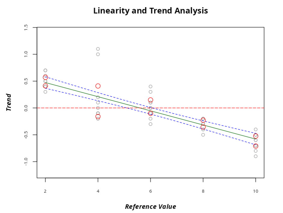
A tendência é considerada significativa ao nível 0.05 para os valores de referência 2.8 e 10. pois o 0 não se encontra entre os limites de confiança.
Linearity is also considered significant at the 0.05 level, as the p-value is less than 0.05, which can also be seen in the Trend graph.
Example 3:
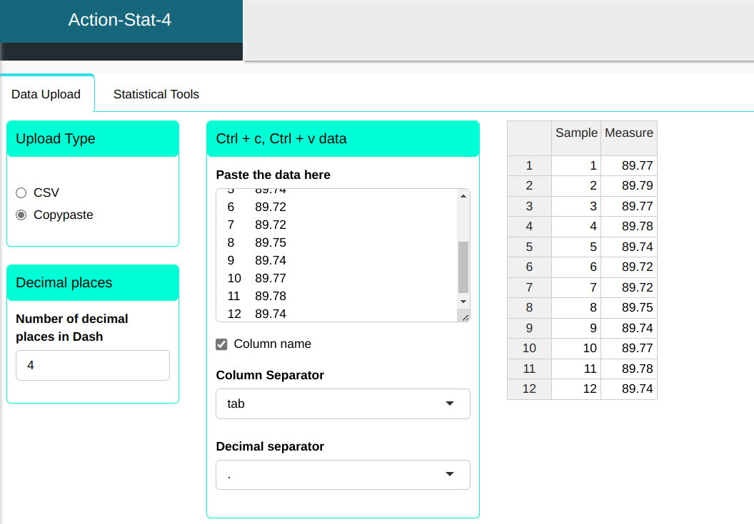
We are going to evaluate the tendency of a measuring system to measure the height of an “MP3 Player”. This height is measured with an altimeter. An “MP3 Player” was selected (close to the nominal value) and its reference value was established with a coordinate measuring system. in which VR = 89.73 mm. and we have a tolerance of 0.7mm. The same “MP3 Player” was then measured 12 times with the measuring system under analysis.
| Sample | Measurement |
|---|---|
| 1 | 89.77 |
| 2 | 89.79 |
| 3 | 89.77 |
| 4 | 89.78 |
| 5 | 89.74 |
| 6 | 89.72 |
| 7 | 89.72 |
| 8 | 89.75 |
| 9 | 89.74 |
| 10 | 89.77 |
| 11 | 89.78 |
| 12 | 89.74 |
We will upload the data to the system.
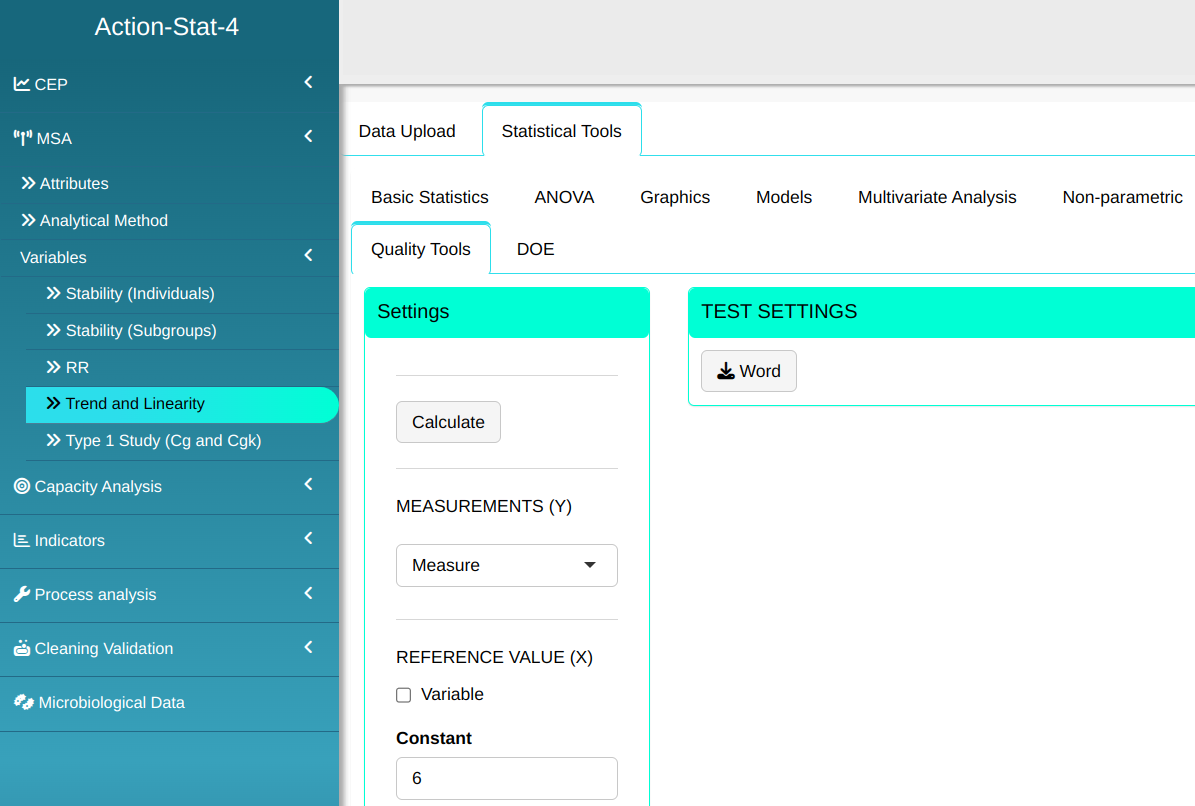
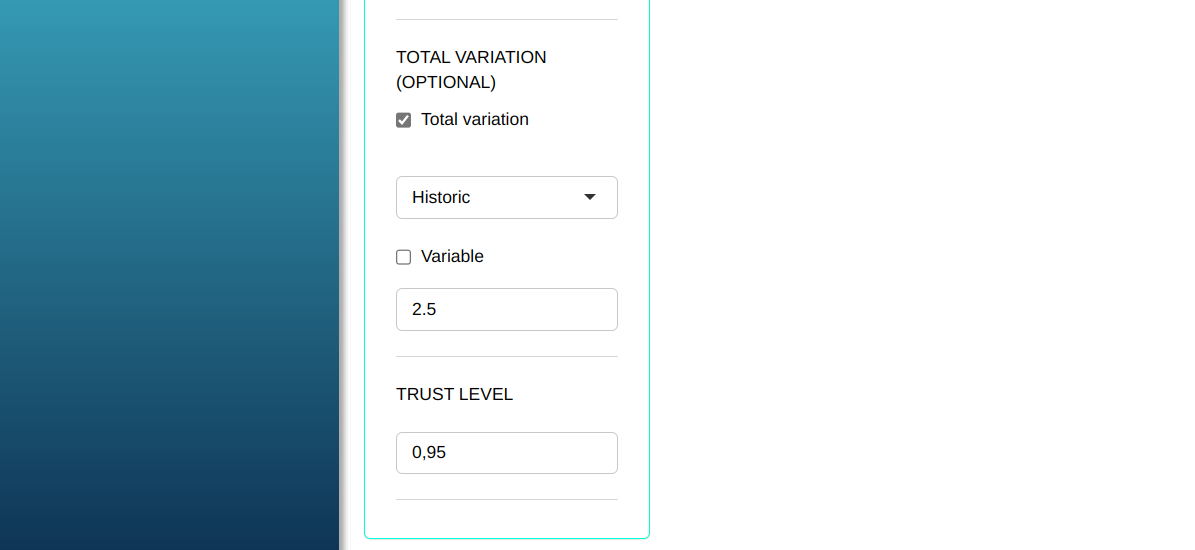
Configuring as shown in the figure below to perform the analysis.
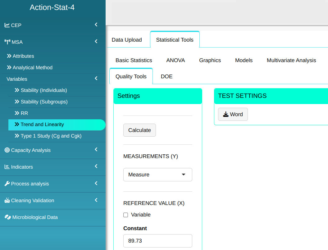
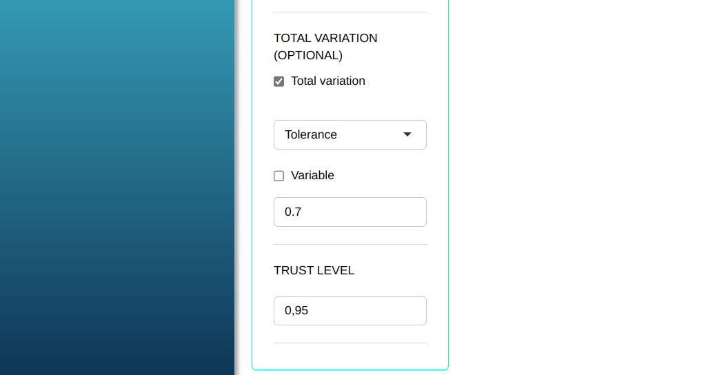
Then click Calculate to get the results. You can also generate the analyses and download them in Word format.
The results are:
TREND ANALYSIS - t TEST
| V1 | |
|---|---|
| Reference value | 89.730 |
| Mean | 89.756 |
| Trend | 0.026 |
| t Statistic | 3.742 |
| P-value | 0.003 |
| Lower Limit | 0.011 |
| Upper Limit | 0.041 |
| EV % | 20.499 |
| Standard Deviation | 0.024 |
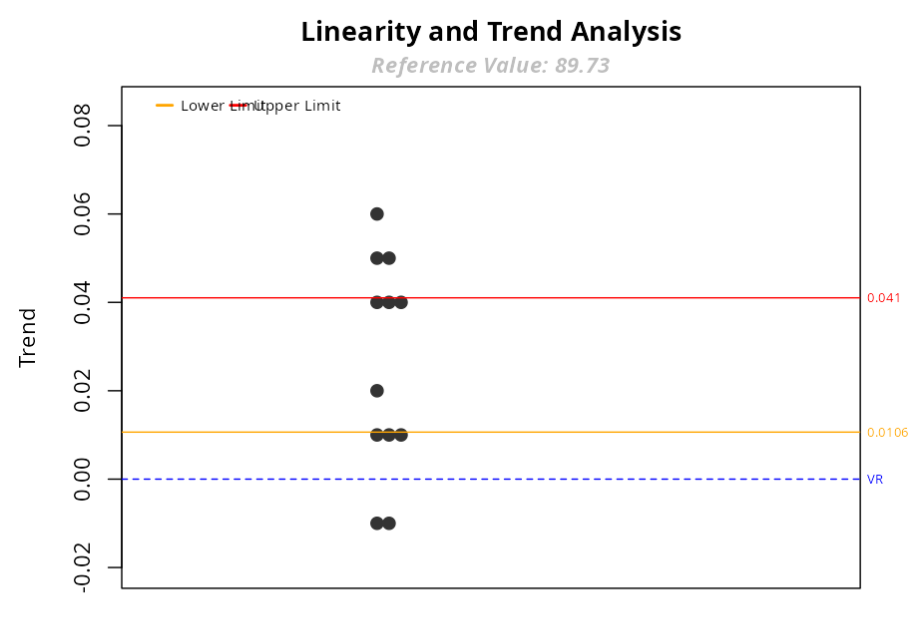
The trend is considered significant at the 0.95 level, as 0 is not within the confidence limits.
The trend graphic also shows that many points has a tendency outside these limits.
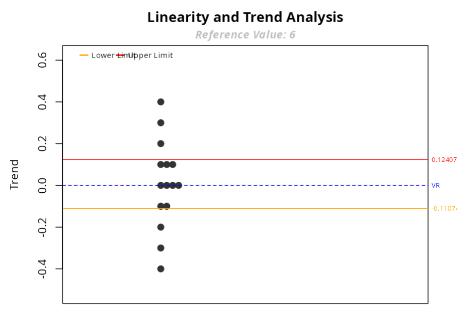
Example 4:
An engineer is evaluating a new measurement system to monitor a process. An analysis of the measurement system indicated that there should be no concern about linearity, as the range of interest is small. A single part has been chosen so that it is close to the nominal value of the processes. The part was measured by a sophisticated measuring system to determine its reference value (reference value = 6). The part was then measured 15 times by an operator and the total process variability value is 2.5, this value will be used to validate the repeatability of the measurement system.
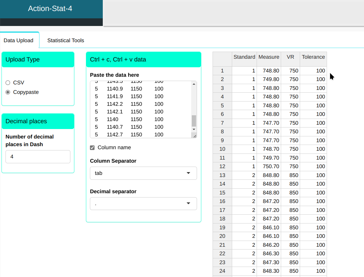
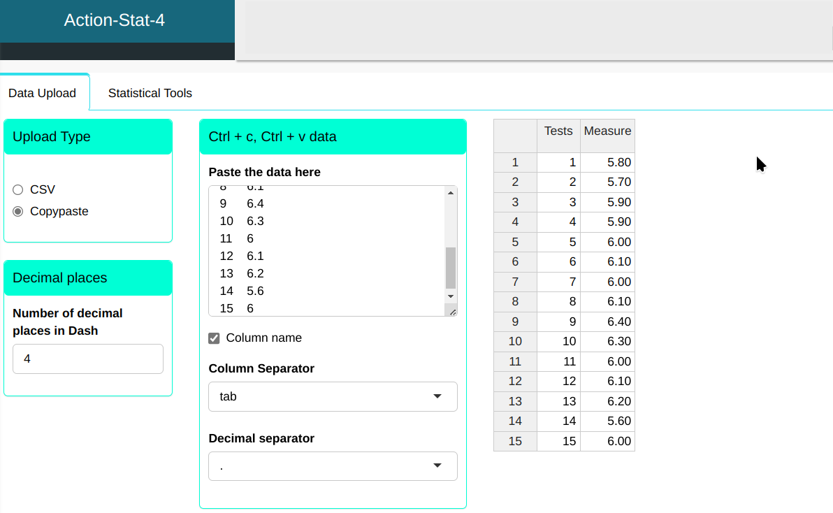
We will upload the data to the system.
| Test | Measurement |
|---|---|
| 1 | 5.8 |
| 2 | 5.7 |
| 3 | 5.9 |
| 4 | 5.9 |
| 5 | 6 |
| 6 | 6.1 |
| 7 | 6 |
| 8 | 6.1 |
| 9 | 6.4 |
| 10 | 6.3 |
| 11 | 6 |
| 12 | 6.1 |
| 13 | 6.2 |
| 14 | 5.6 |
| 15 | 6 |
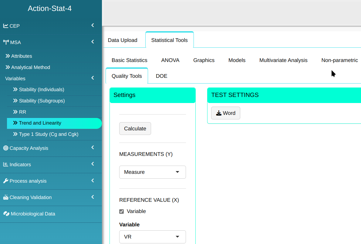
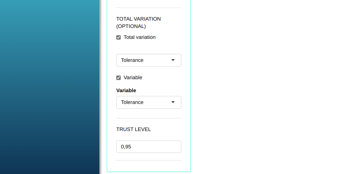
Configuring as shown in the figure below to perform the analysis.
Then click Calculate to get the results. You can also generate the analyses and download them in Word format.
The results are:
ANÁLISE DE TENDÊNCIA - Teste t
| V1 | |
|---|---|
| Reference value | 6.000 |
| Mean | 6.007 |
| Trend | 0.007 |
| Statistic | 0.122 |
| P-value | 0.905 |
| Lower Limit | -0.111 |
| Upper Limit | 0.124 |
| EV % | 8.481 |
| Standard Deviation | 0.212 |