3. Dotplot
Dotplot represents each observation obtained on a horizontal scale, allowing visualization of the distribution of data during this time. Furthermore, it allows visual comparison of the two data sets.
Example 1:
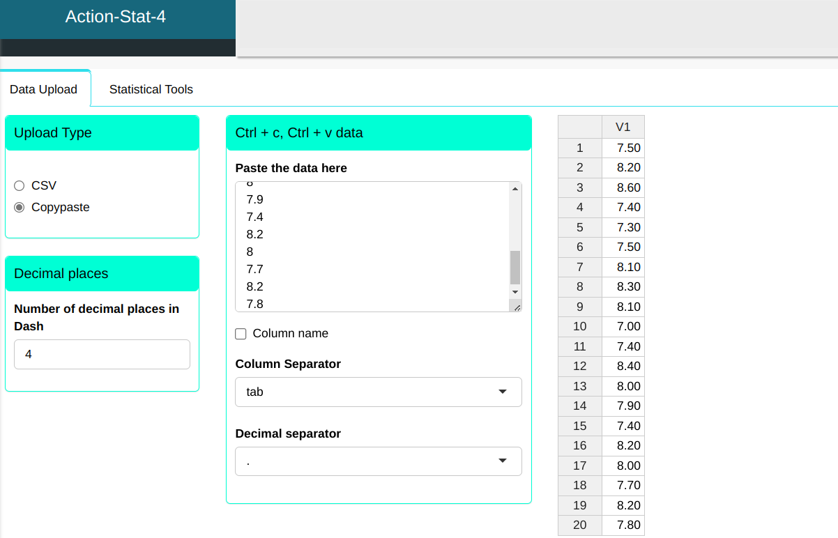
We will upload the measurement of 20 iron bars to the system.
| 7.5 |
| 8.2 |
| 8.6 |
| 7.4 |
| 7.3 |
| 7.5 |
| 8.1 |
| 8.3 |
| 8.1 |
| 7 |
| 7.4 |
| 8.4 |
| 8 |
| 7.9 |
| 7.4 |
| 8.2 |
| 8 |
| 7.7 |
| 8.2 |
| 7.8 |
The Dotplot graph is created according to the configuration shown in the figure below.
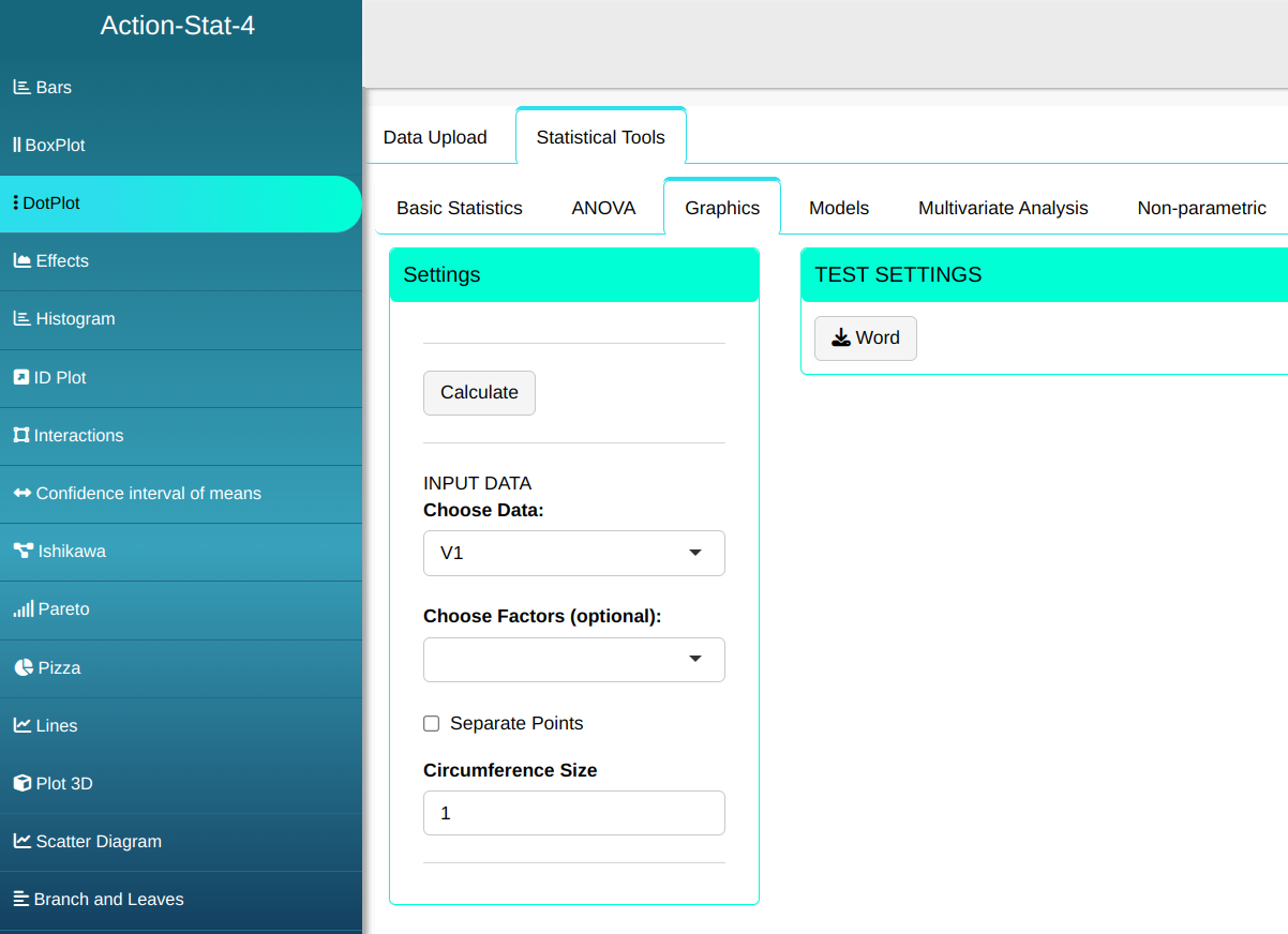
Click on calculate to view the results and download them in a Word document.
The results are:
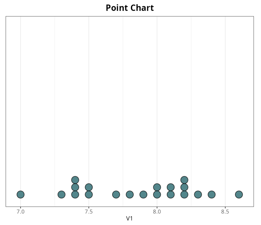
The lengths of the iron bars are concentrated between the values 7.0 and 8.5 so that the dispersion between the values is small in relation to the average of the values.
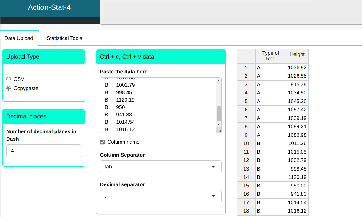
Example 2:
Let us consider the example given previously: two types of rods, A and B. Make a Dotplot and compare the two types of rod.
| Type of Rod | Height |
|---|---|
| A | 1036.92 |
| A | 1026.58 |
| A | 915.38 |
| A | 1034.50 |
| A | 1045.20 |
| A | 1057.42 |
| A | 1039.19 |
| A | 1099.21 |
| A | 1086.98 |
| B | 1011.26 |
| B | 1015.05 |
| B | 1002.79 |
| B | 998.45 |
| B | 1120.19 |
| B | 950.00 |
| B | 941.83 |
| B | 1014.54 |
| B | 1016.12 |
We will upload the data to the system.
The Dotplot graph is created according to the configuration shown in the figure below.
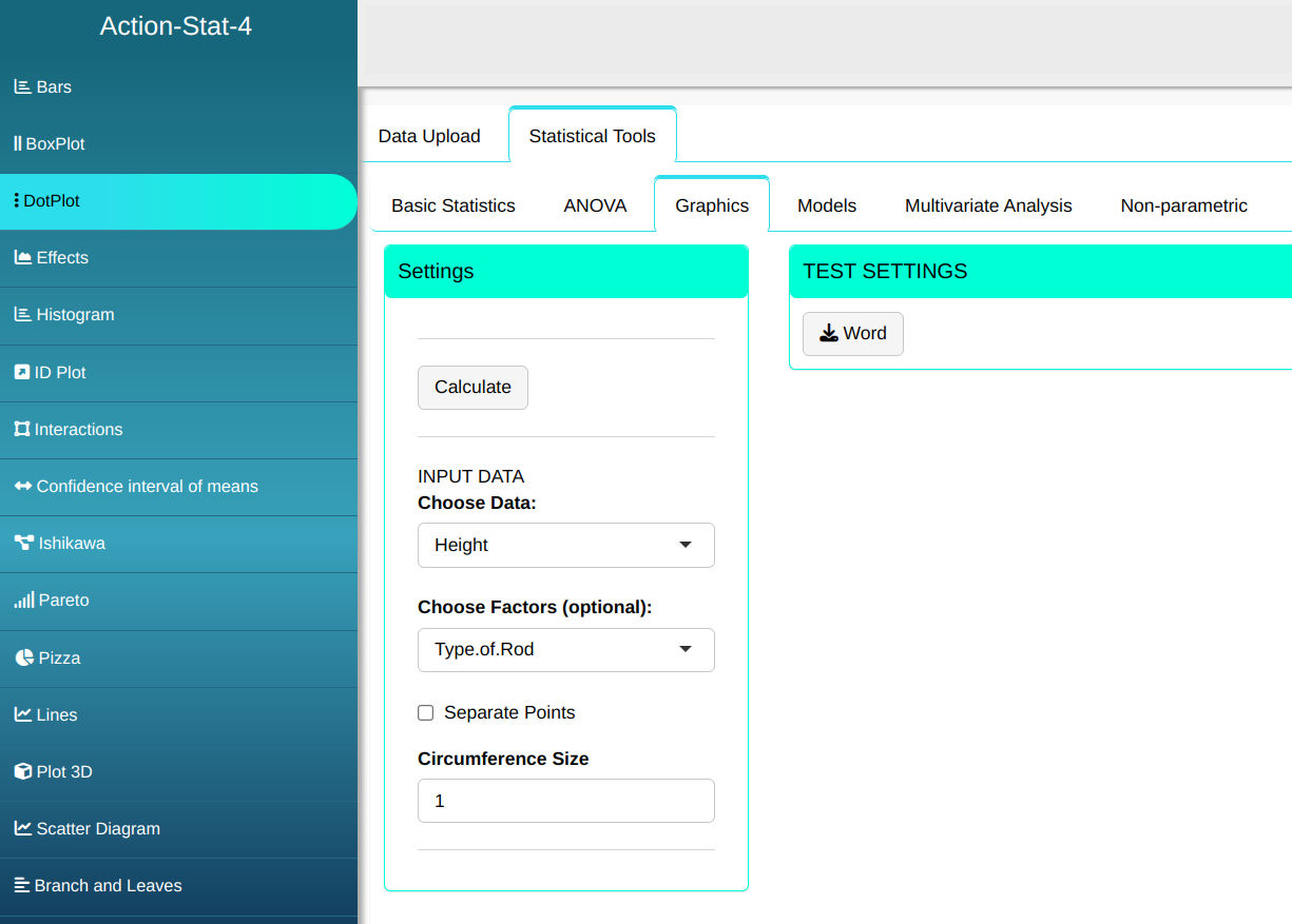
Click on calculate to view the results and download them in a Word document.
The results are:
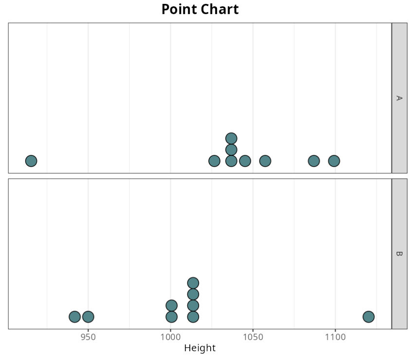
Comparing the two types of rods, we notice slightly higher heights. tops of the type A rods, although one of them still has a height much lower than type B measurements.