5. Histogram

Histogram is a graphical representation (a vertical bar graph) the frequency distribution of a set of quantitative data continuous.

Example:

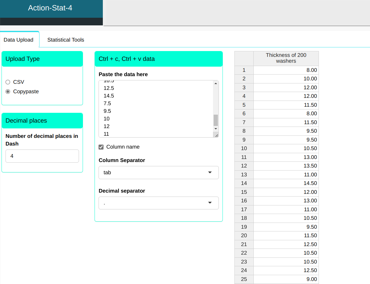
In an auto parts factory, a sealing washer was causing inconvenient when assembling a part of a car. To search information, we decided to measure the thickness of 200 washers, whose values they were:

Thickness of 200 washers
8
10
12
12
11.5
8
11.5
9.5
9.5
10.5
13
13.5
11
14.5
12
13
11
10.5
9.5
11.5
12.5
10.5
10.5
12.5
9
13
11.5
14.5
13.5
12.5
10
10.5
8
13
7
8
7
7
9.5
11.5
12.5
8
13.5
15.5
9.5
15
10
10
9
14.5
11
10.5
11.5
8.5
8
10
7.5
10
12.5
8
14
15
11.5
13.5
11.5
9.5
12.5
5
8
13
8.5
7.5
10
11
13.5
9
15.5
12.5
7
10.5
13.5
9
12
12.5
12.5
12.5
9
13.5
12.5
12.5
10.5
8
8.5
13.5
13
13
13
9.5
9.5
14.5
12
13
15.5
17
14
15
13
7.5
12
12
7
12.5
10.5
8.5
6
15
15.5
10
12
8.5
14
11
14
8
11.5
13.5
11.5
11
9.5
13
10
10.5
12
11
10
10
11.5
10
10
10
12
10
7.5
11
13
12
16
9
10
8.5
12
14.5
10.5
11
10
13.5
10.5
12
10
12.5
10
14
11.5
11.5
13
11
10.5
10.5
7.5
10.5
12
12
11
10
12
11.5
9.5
8.5
8.5
12.5
14.5
11
11
17
15
11
9
14
10.5
10.5
10.5
8
10.5
12.5
14.5
7.5
9.5
10
12
11

---

We will upload the system data.

We will make the Histogram.

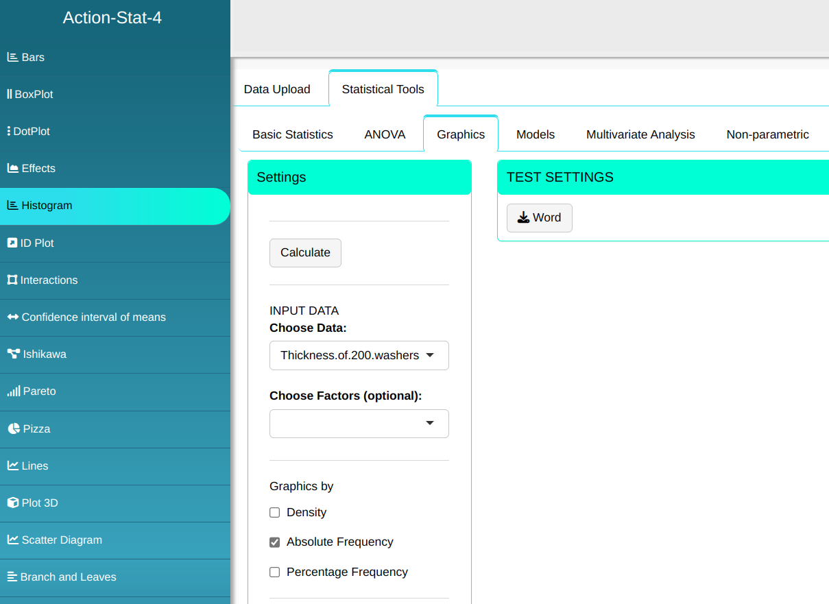
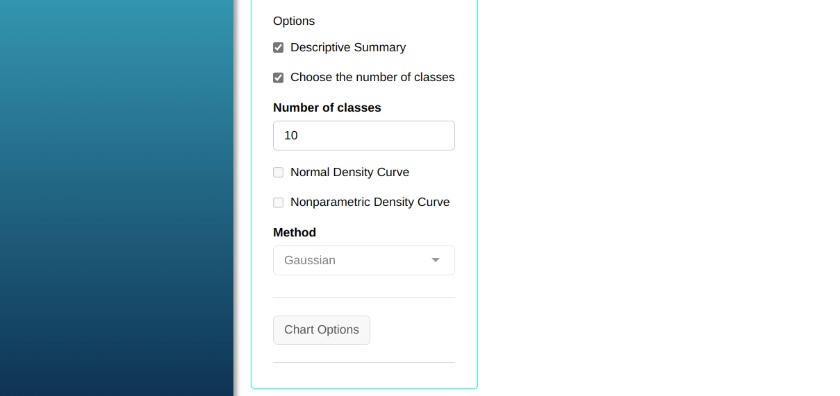
Then click Calculate to get the results. You can also generate the analyses and download them in Word format.

The results are:

Frequency Table

Class	Frequency	Rel. Freq.	Perc. Freq.	Cum. Freq.	Density	Median Point
[5; 6.2)	2	0.01	1.0	1.0	0.008	5.6
[6.2; 7.4)	5	0.02	2.5	3.5	0.021	6.8
[7.4; 8.6)	25	0.12	12.5	16.0	0.104	8.0
[8.6; 9.8)	18	0.09	9.0	25.0	0.075	9.2
[9.8; 11)	40	0.20	20.0	45.0	0.167	10.4
[11; 12,2)	46	0.23	23.0	68.0	0.192	11.6
[12.2; 13.4)	29	0.14	14.5	82.5	0.121	12.8
[13.4; 14.6)	23	0.12	11.5	94.0	0.096	14.0
[14.6; 15.8)	9	0.04	4.5	98.5	0.038	15.2
[15.8; 17)	3	0.02	1.5	100.0	0.012	16.4

---

Descriptive Summary

	Values ​​
Minimum	5.000
1° Quartile	9.625
Median	11.000
Mean	11.152
3° Quartile	12.500
Maximum	17.000
Standard Deviation	2.249

---

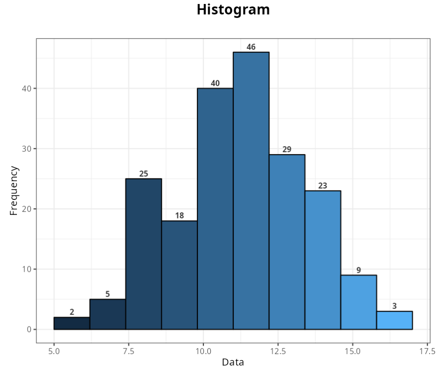
From the histogram we see that the washer thicknesses follow, approximately, a normal distribution, with the measures concentrated close to the mean (between 9 and 11 mm).