8. Confidence Interval of means
A simple estimate of the mean gives no idea of how close or far away from its true value, or rather the accuracy of the result. Therefore, a common method of specifying this precision is to determine a confidence interval for the population parameter.
Example 1:
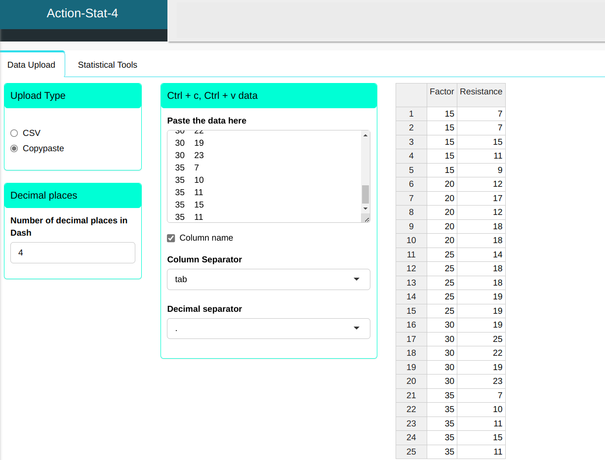
Let’s consider a data set with one factor and several levels. upload the set to the system.
| Factor | Resistance |
|---|---|
| 15 | 7 |
| 15 | 7 |
| 15 | 15 |
| 15 | 11 |
| 15 | 9 |
| 20 | 12 |
| 20 | 17 |
| 20 | 12 |
| 20 | 18 |
| 20 | 18 |
| 25 | 14 |
| 25 | 18 |
| 25 | 18 |
| 25 | 19 |
| 25 | 19 |
| 30 | 19 |
| 30 | 25 |
| 30 | 22 |
| 30 | 19 |
| 30 | 23 |
| 35 | 7 |
| 35 | 10 |
| 35 | 11 |
| 35 | 15 |
| 35 | 11 |
We use the Confidence Interval of Means tool.


Then click Calculate to get the results. You can also generate the analyses and download them in Word format.

The results are:
Confidence Interval for the Mean
| Mean | Standard Deviation | Lower Limit | Upper Limit | |
|---|---|---|---|---|
| 1 | 9.8 | 2.839 | 7.152 | 12.448 |
| 2 | 15.4 | 2.839 | 12.752 | 18.048 |
| 3 | 17.6 | 2.839 | 14.952 | 20.248 |
| 4 | 21.6 | 2.839 | 18.952 | 24.248 |
| 5 | 10.8 | 2.839 | 8.152 | 13.448 |
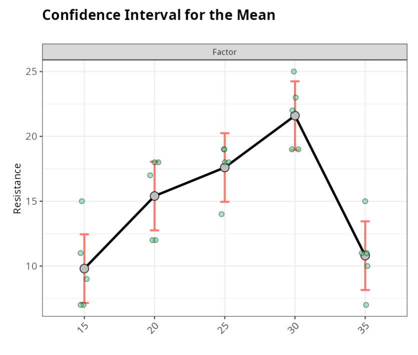
In the graph, and also in the table, we have the mean of each level and the respective confidence intervals. We can see that the five factors differ in terms of their resistance, since factor 30 has relatively higher results than the others.
Example 2:
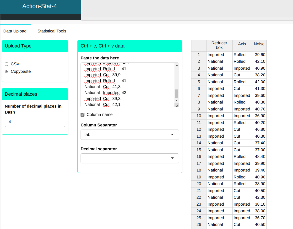
Let’s consider a data set with two factors (Gearbox and Axle) and several levels, as shown in the table below.
| Reducer box | Axis | Noise |
|---|---|---|
| Imported | Rolled | 39.6 |
| National | Rolled | 42.1 |
| National | Imported | 40.9 |
| National | Cut | 38.2 |
| National | Rolled | 42 |
| Imported | Cut | 41.3 |
| Imported | Imported | 39.6 |
| National | Rolled | 40.3 |
| National | Imported | 40.7 |
| Imported | Imported | 36.9 |
| Imported | Rolled | 40.2 |
| Imported | Cut | 46.8 |
| Imported | Cut | 40.3 |
| National | Cut | 37.4 |
| National | Cut | 37 |
| Imported | Rolled | 48.4 |
| Imported | Imported | 39.9 |
| National | Imported | 39.4 |
| Imported | Rolled | 40.9 |
| National | Rolled | 38.9 |
| Imported | Cut | 40.5 |
| National | Cut | 42.3 |
| Imported | Imported | 38.1 |
| Imported | Imported | 38 |
| Imported | Imported | 36.7 |
| National | Cut | 40.5 |
| National | Rolled | 38.9 |
| Imported | Imported | 37.2 |
| Imported | Rolled | 39.9 |
| National | Rolled | 43.7 |
| National | Imported | 41.4 |
| National | Rolled | 41 |
| Imported | Cut | 41.3 |
| National | Imported | 41.3 |
| Imported | Imported | 36.7 |
| National | Rolled | 40.1 |
| National | Cut | 41.3 |
| Imported | Rolled | 41 |
| National | Imported | 40.6 |
| National | Cut | 40.4 |
| National | Rolled | 40.3 |
| National | Imported | 41.3 |
| Imported | Cut | 40.1 |
| Imported | Rolled | 42.7 |
| Imported | Cut | 41.6 |
| National | Imported | 41.6 |
| Imported | Imported | 36.2 |
| Imported | Rolled | 41 |
| Imported | Cut | 39.9 |
| Imported | Rolled | 41 |
| National | Cut | 41.3 |
| National | Imported | 42 |
| Imported | Cut | 39.3 |
| National | Cut | 42.1 |
We will upload the data to the system.
We use the Confidence Interval of Means tool.
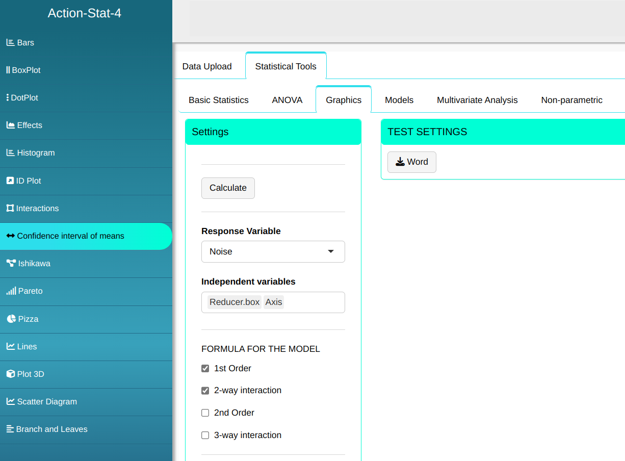

Then click Calculate to get the results. You can also generate the analyses and download them in Word format.
The results are:
Intervalo de Confiança das Médias
| Mean | Standard Deviation | Lower Limit | Upper Limit | |
|---|---|---|---|---|
| 1 | 40.1889 | 2.1172 | 39.3705 | 41.0073 |
| 2 | 40.6296 | 2.1172 | 39.8112 | 41.448 |
Confidence Interval for the Mean
| Mean | Standard Deviation | Lower Limit | Upper Limit | |
|---|---|---|---|---|
| 1 | 40.6444 | 2.1172 | 39.6421 | 41.6468 |
| 2 | 39.3611 | 2.1172 | 38.3588 | 40.3635 |
| 3 | 41.2222 | 2.1172 | 40.2199 | 42.2246 |
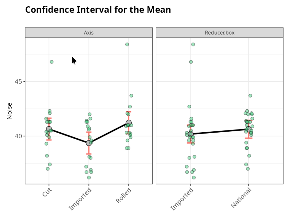
In the graph, and also in the table, we have the mean for each level and the respective confidence intervals. Here we see that regardless of the factors and their respective levels, the noise behaves in a very similar way, with the exception of when the imported axis is considered, where then the noise decreases on average.