6. ID Plot

Way to verify, through probability paper, a distribution which best describes the randomness of a data set.

Example:

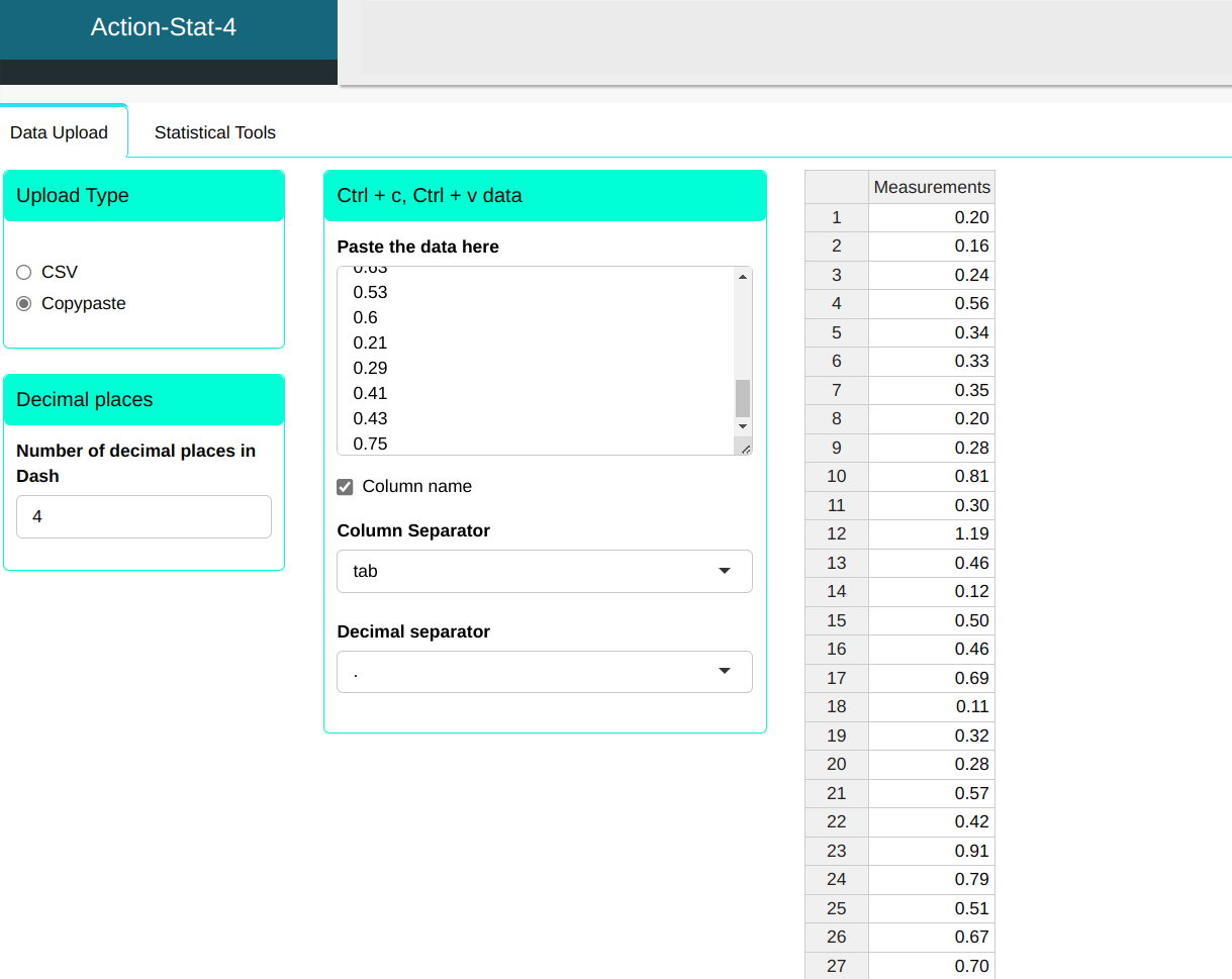
We consider the dataset in the following table. Let’s check Which probability distribution best describes this set of data.

---

Medicines
0.20
0.16
0.24
0.56
0.34
0.33
0.35
0.20
0.28
0.81
0.30
1.19
0.46
0.12
0.50
0.46
0.69
0.11
0.32
0.28
0.57
0.42
0.91
0.79
0.51
0.67
0.70
0.19
0.22
0.62
0.56
0.96
0.11
0.85
0.37
0.80
0.52
0.17
0.58
0.15
0.20
0.05
0.63
0.53
0.60
0.21
0.29
0.41
0.43
0.75

---

We will upload the data to the system.

Configuring according to the figure below and we will do the ID plot

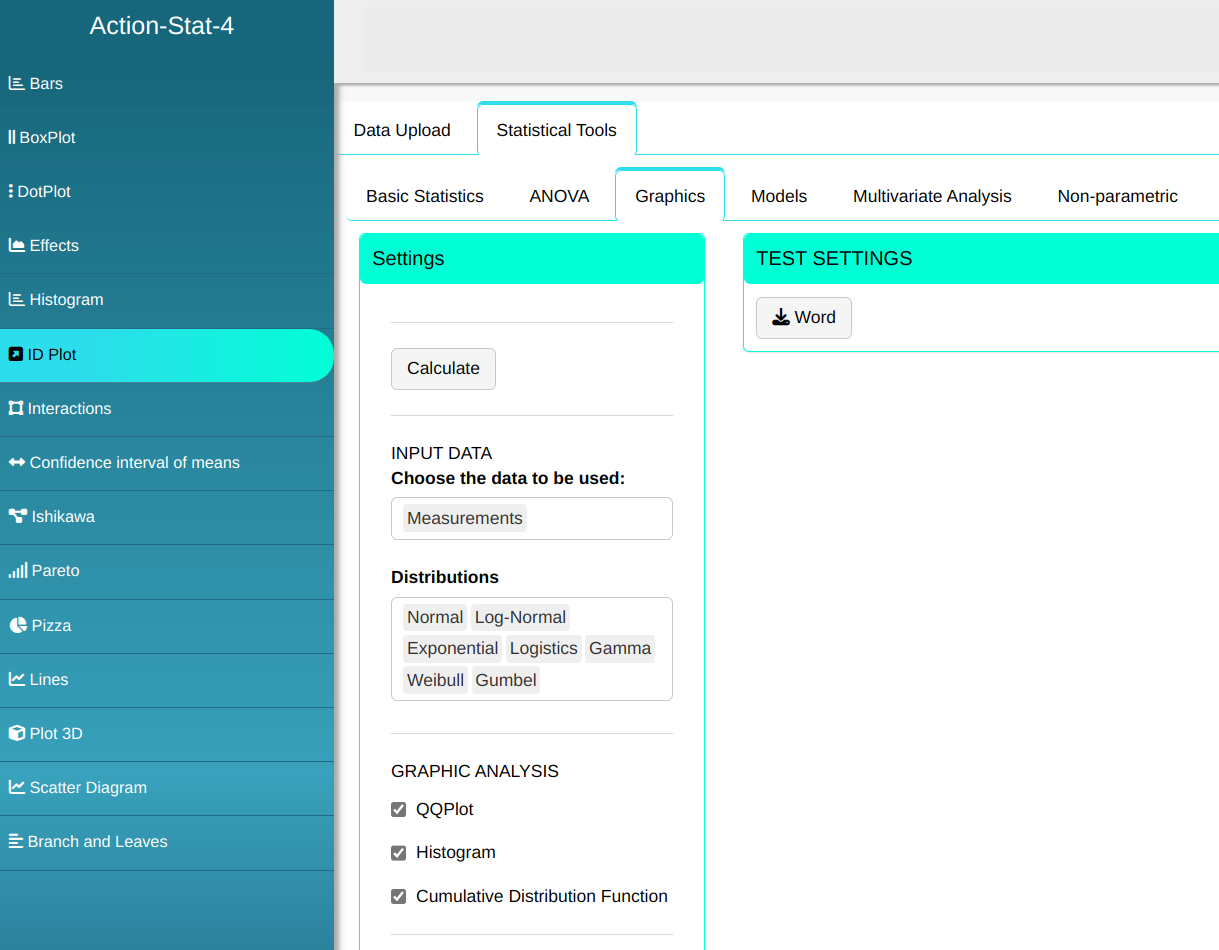
Then click Calculate to get the results. You can also generate the analyses and download them in Word format.

The results are:

Analysis result

		Box-Cox Transformation

---

Results

	Values
Lambda	0.429
P-Value (Anderson-Darling)	0.703

---

Analysis result

		Johnson Transformation

---

Estimates

	test
Gamma	0.90802942754439
Lambda	1.36936290670753
Epsilon	0.0168457063069285
Eta	0.951739827664239
Family	SB
P-Value (Anderson-Darling)	0.9422

---

Anderson-Darling

	Distributions	Statistics	P-Value
1	Normal( $\mu$ = 0.45, $\sigma$ = 0.26)	0.566	0.136
2	Log-Normal(log($\mu$) = -0.982398, log($\sigma$) = 0.667801)	0.589	0.118
1-mle-exp	Exponential(Rate = 2.20556)	3,845	0.000
11	Logistics(Location = 0.44, Scale = 0.15)	0.581	0.089
12	Gamma(Shape = 2.76743, Rate = 6.10372)	0.295	0.250
13	Weibull(Shape = 1.84755, Scale = 0.511436)	0.217	0.250
14	Gumbel(Location = 0.332819, Scale = 0.207431)	0.384	0.250

---

Cramer-von-Misés

Distributions	Statistics	P-Value
Normal($\mu$ = 0.45, $\sigma$ = 0.26)	0.082	0.192
Log-Normal(log($\mu$) = -0.982398, log($\sigma$) = 0.667801)	0.100	0.114
Exponential(Rate = 2.20556)	0.678	0.000
Logistics(Location = 0.44, Scale = 0.15)	0.076	0.232
Gamma(Shape = 2.76743, Rate = 6.10372)	0.051	0.497
Weibull(Shape = 1.84755, Scale = 0.511436)	0.035	0.765
Gumbel(Location = 0.332819, Scale = 0.207431)	0.065	0.329

---

Kolmogorov-Smirnov

Distributions	Statistics	P-Value
Normal($\mu$ = 0.45, $\sigma$ = 0.26)	0.095	0.313
Log-Normal(log($\mu$) = -0.982398, log($\sigma$) = 0.667801)	0.108	0.158
Exponential(Rate = 2.20556)	0.202	0.000
Logistics(Location = 0.44, Scale = 0.15)	0.082	0.550
Gamma(Shape = 2.76743, Rate = 6.10372)	0.083	0.534
Weibull(Shape = 1.84755, Scale = 0.511436)	0.070	0.778
Gumbel(Location= 0.332819, Scale = 0.207431)	0.081	0.559

---

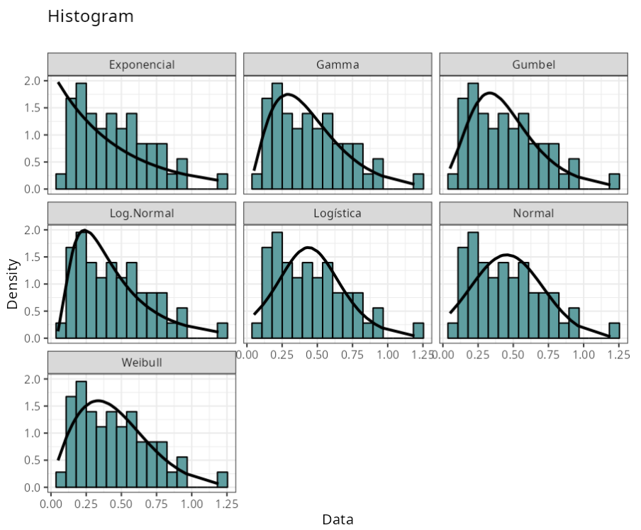
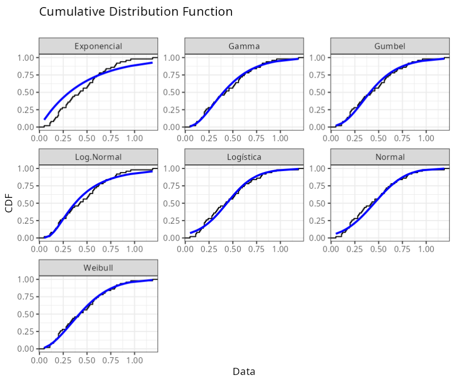
Analysis result

		Graphic Analysis

---

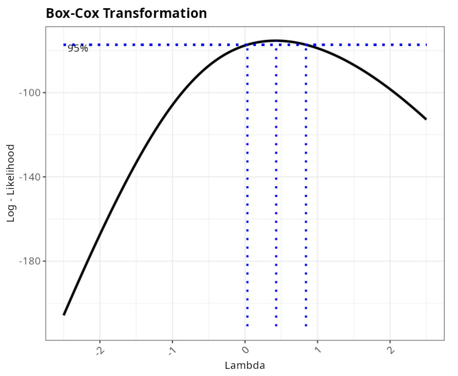
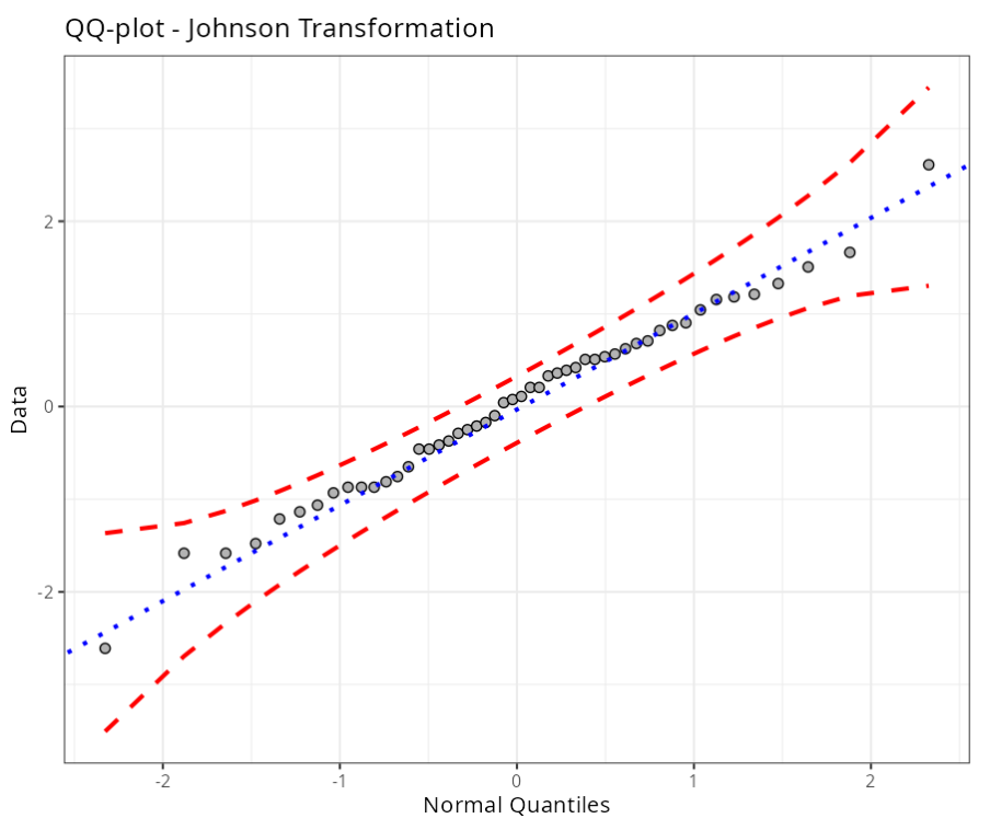
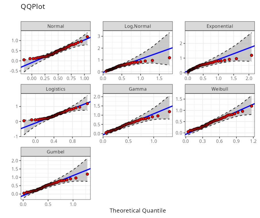
Data transformed using Box-Cox Transformation and Johnson transformations follow a normal distribution. This result can be confirmed by observing the p-value associated with the Anderson-Darling.

The table indicates that the data can be better fitted by all distributions except Exponential Distribution, which can be confirmed when we compare the p-value of the Anderson-Darling test with the level of significance of 0.05.