1. Simple Linear Model

The simple linear model is used to analyze the relationship between two or more variables.

Example:

In heat treatment problems, you want to establish a relationship between the temperature of the oven and a quality characteristic (hardness) of a part.

---

Hardness	Temperature
137	220
137	220
137	220
136	220
135	220
135	225
133	225
132	225
133	225
133	225
128	230
124	230
126	230
129	230
126	230
122	235
122	235
122	235
119	235
122	235

---

We will upload the data to the system.

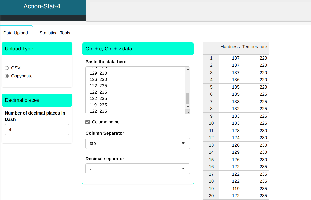
Configuring according to the figure below to perform the analysis.

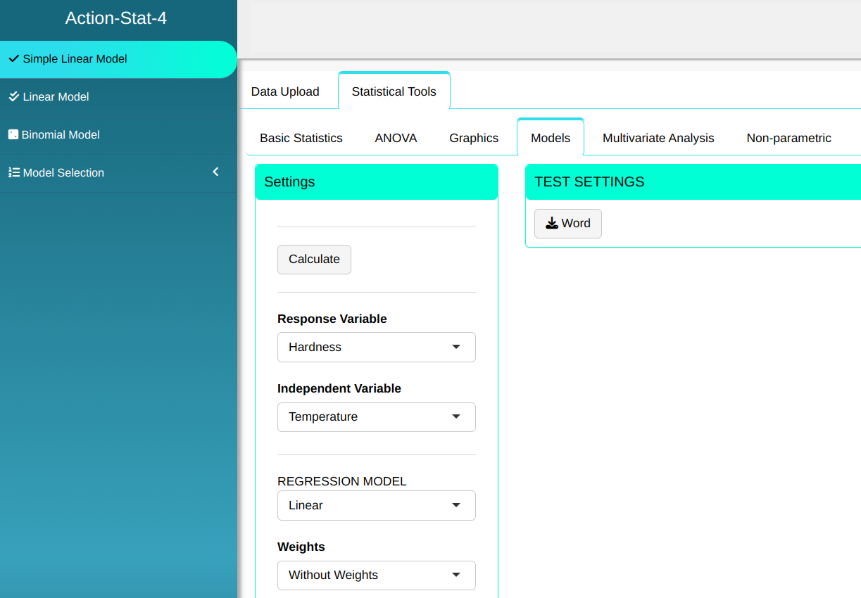
Then click Calculate to get the results. You can also generate the analyses and download them in Word format.

The results are

ANOVA Table

	D.F.	Sum of Squares	Mean Squares	F.Stat.	P-Value
Temperature	1	665.64	665.640000	291.0962	0
Residuals	18	41.16	2.286667

---

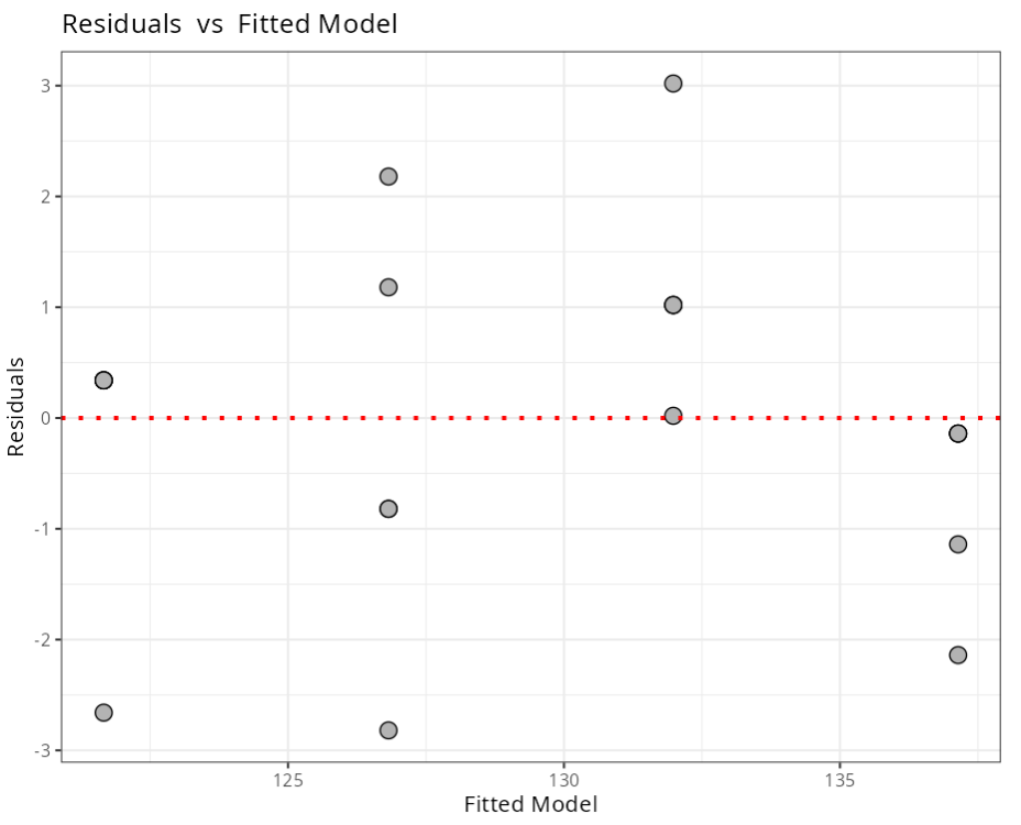
Exploratory Analysis (residues)

Minimum	1Q	Median	Mean	3Q	Maximum
-2.82	-0.82	0.18	0	1.02	3.02

---

Coefficients

	Estimate	Standard Deviation	T Stat.	P-Value
Intercept	364.180	13.76492644	26.45710	0
Temperature	-1.032	0.06048691	-17.06154	0

---

Descriptive measure for Goodness-of-Fit

Standard Deviation of residuals	Degrees of Freedom	$R^2$	Adjusted $R^2$
1.512173	18	0.9417657	0.9385305

–

Confidence Interval for the parameters

	2.5 %	97.5 %
Intercept	335.260963	393.0990373
Temperature	-1.159078	-0.9049217

Prediction Interval

	Hardness	Temperature	Fitted Value	Lower Limit	Upper Limit	Standard Deviation
1	137	220	137.14	135.9513	138.3287	0.5658033
2	137	220	137.14	135.9513	138.3287	0.5658033
3	137	220	137.14	135.9513	138.3287	0.5658033
4	136	220	137.14	135.9513	138.3287	0.5658033
5	135	220	137.14	135.9513	138.3287	0.5658033
6	135	225	131.98	131.2018	132.7582	0.3704052
7	133	225	131.98	131.2018	132.7582	0.3704052
8	132	225	131.98	131.2018	132.7582	0.3704052
9	133	225	131.98	131.2018	132.7582	0.3704052
10	133	225	131.98	131.2018	132.7582	0.3704052
11	128	230	126.82	126.0418	127.5982	0.3704052
12	124	230	126.82	126.0418	127.5982	0.3704052
13	126	230	126.82	126.0418	127.5982	0.3704052
14	129	230	126.82	126.0418	127.5982	0.3704052
15	126	230	126.82	126.0418	127.5982	0.3704052
16	122	235	121.66	120.4713	122.8487	0.5658033
17	122	235	121.66	120.4713	122.8487	0.5658033
18	122	235	121.66	120.4713	122.8487	0.5658033
19	119	235	121.66	120.4713	122.8487	0.5658033
20	122	235	121.66	120.4713	122.8487	0.5658033

Forecast Interval

Temperature	Fitted Value	Lower Limit	Upper Limit	Standard Deviation
220	137.14	133.7479	140.5321	1.512173
220	137.14	133.7479	140.5321	1.512173
220	137.14	133.7479	140.5321	1.512173
220	137.14	133.7479	140.5321	1.512173
220	137.14	133.7479	140.5321	1.512173
225	131.98	128.7091	135.2509	1.512173
225	131.98	128.7091	135.2509	1.512173
225	131.98	128.7091	135.2509	1.512173
225	131.98	128.7091	135.2509	1.512173
225	131.98	128.7091	135.2509	1.512173
230	126.82	123.5491	130.0909	1.512173
230	126.82	123.5491	130.0909	1.512173
230	126.82	123.5491	130.0909	1.512173
230	126.82	123.5491	130.0909	1.512173
230	126.82	123.5491	130.0909	1.512173
235	121.66	118.2679	125.0521	1.512173
235	121.66	118.2679	125.0521	1.512173
235	121.66	118.2679	125.0521	1.512173
235	121.66	118.2679	125.0521	1.512173
235	121.66	118.2679	125.0521	1.512173

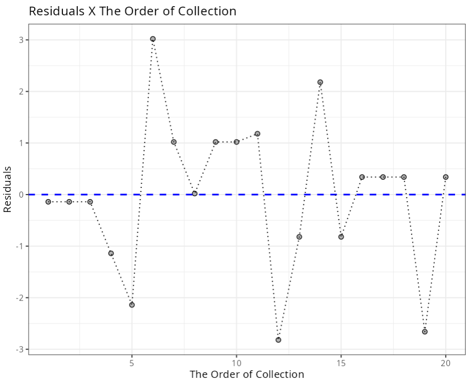
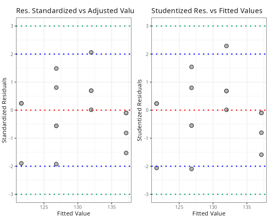
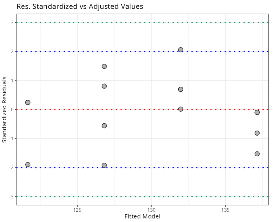
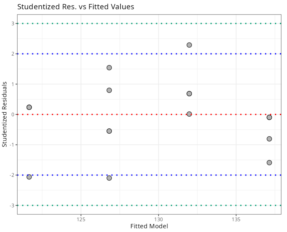
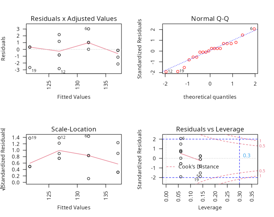
Summary of Residual Analysis

N.Obs	Hardness	Temperature	Residuals	Studentized Residuals	Standardized Residuals	Leverage	DFFITS	DFBETA
1	137	220	-0.14	-0.09704784	-0.09983375	0.14	-0.039156210	0.031394812
2	137	220	-0.14	-0.09704784	-0.09983375	0.14	-0.039156210	0.031394812
3	137	220	-0.14	-0.09704784	-0.09983375	0.14	-0.039156210	0.031394812
4	136	220	-1.14	-0.80494250	-0.81293195	0.14	-0.324772801	0.260397546
5	135	220	-2.14	-1.58941025	-1.52603016	0.14	-0.641284585	0.514171544
6	135	225	3.02	2.28984318	2.05987841	0.06	0.578518751	-0.236179291
7	133	225	1.02	0.68539691	0.69572052	0.06	0.173162497	-0.070693294
8	132	225	0.02	0.01325730	0.01364158	0.06	0.003349398	-0.001367386
9	133	225	1.02	0.68539691	0.69572052	0.06	0.173162497	-0.070693294
10	133	225	1.02	0.68539691	0.69572052	0.06	0.173162497	-0.070693294
11	128	230	1.18	0.79664291	0.80485315	0.06	0.201268307	0.082167442
12	124	230	-2.82	-2.09718028	-1.92346262	0.06	-0.529843321	-0.216307630
13	126	230	-0.82	-0.54833211	-0.55930473	0.06	-0.138533682	-0.056556139
14	129	230	2.18	1.54290019	1.48693210	0.06	0.389806907	0.159138003
15	126	230	-0.82	-0.54833211	-0.55930473	0.06	-0.138533682	-0.056556139
16	122	235	0.34	0.23600803	0.24245339	0.14	0.095222937	0.076348201
17	122	235	0.34	0.23600803	0.24245339	0.14	0.095222937	0.076348201
18	122	235	0.34	0.23600803	0.24245339	0.14	0.095222937	0.076348201
19	119	235	-2.66	-2.06083935	-1.89684123	0.14	-0.831493637	-0.666678066
20	122	235	0.34	0.23600803	0.24245339	0.14	0.095222937	0.076348201

---

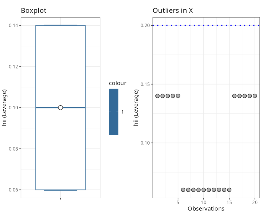
Criterion

Diagnostic	Formula	Value
hii (Leverage)	(2*(p+1))/n	0.20
DFFITS	2* raíz ((p+1)/n)	0.63
DCOOK	4/n	0.20
DFBETA	2/raíz(n)	0.45
Standardized Resíduals	(-3,3)	3.00
Studentized Residuals	(-3,3)	3.00

---

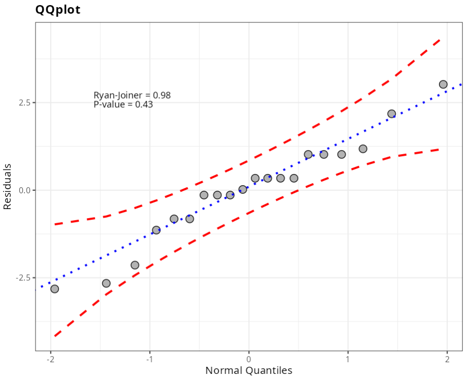
Normality Test

	Statistics	P-value
Anderson-Darling	0.4053853	0.3202935
Shapiro-Wilk	0.9594731	0.5333777
Kolmogorov-Smirnov	0.1621102	0.1827284
Ryan-Joiner	0.9785600	0.4164000

---

Homoscedasticity Test - Cochran

Statistics	Number of Replicas	P-Value
0.5	5	0.25

---

Homoscedasticity Test (Brown-Forsythe)

Variable	Statistics	DF.Num.	DF.Den.	P-value
Grupo	0.6153846	3	16	0.6149536

---

Homoscedasticity Test - Breusch Pagan

Statistics	DF	P-value
0.07844525	1	0.7794155

---

Homoscedasticity test - Goldfeld Quandt

Variable	Statistics	DF1	DF2	P-value
Temperature	1.67796610169501	6	6	0.545208843765449

---

*Independence Test - Durbin-Watson

Statistics	P-value
2.235102	0.7686383

---

Lack of Fit Test

	DF	Sum of Squares	Mean Squares	F. Stat.	P-value
Temperature	1	665.64	665.640000	350.336842	0.
Residuals	18	41.16	2.286667
Lack of Fit	2	10.76	5.380000	2.831579	0.088549423924260837
Pure Error	16	30.40	1.900000

---

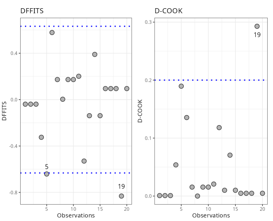
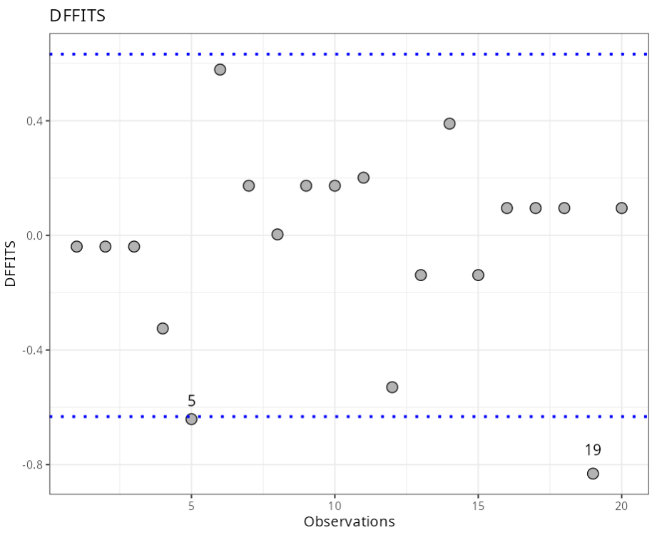
Influential Points

Observations	DFFITS	Criterion
5	-0.64	± 0.63
19	-0.83	± 0.63

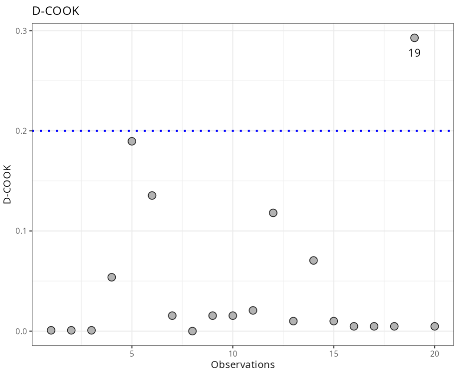
Influential Points

Observations	DCOOK	Criterion
19	0.2929	0.2

---

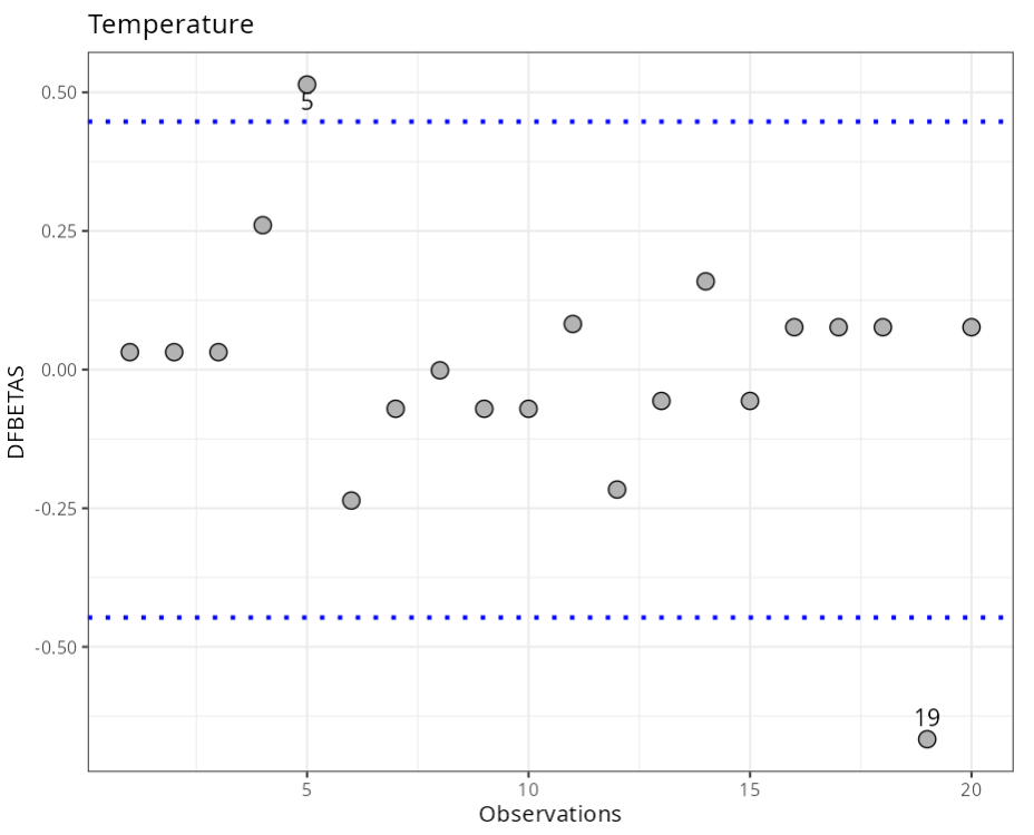
Temperature

Observations	DFBETA	Criterion
5	0.5142	0.4472
19	-0.6667	0.4472

---