3. Binomial Model

The binomial regression model is used when the response variable is variable with two possible outcomes.

Example 1:

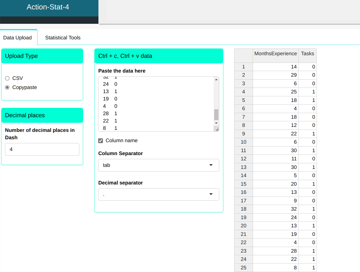
An analyst is studying the effect of length of experience in computer programming on the ability to complete a difficult task within a given time. Twenty-five programmers were selected for the study. The predictor variable, X, corresponds to months of experience.

Observation:

Tasks (Y)=1, whether the task was successfully completed in the time allowed, and

Tasks (Y)=0, if the task was not completed successfully.

MonthsExperience	Tasks
14	0
29	0
6	0
25	1
18	1
4	0
18	0
12	0
22	1
6	0
30	1
11	0
30	1
5	0
20	1
13	0
9	0
32	1
24	0
13	1
19	0
4	0
28	1
22	1
8	1

We will upload the data to the system.

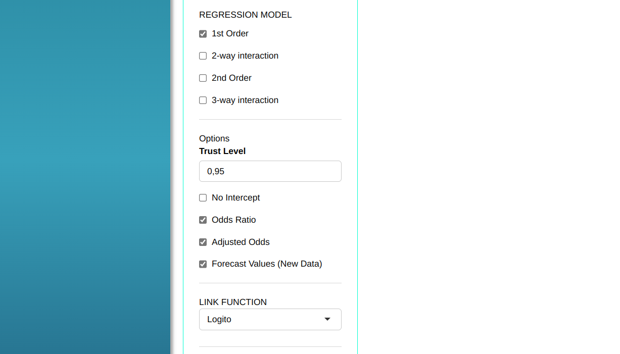
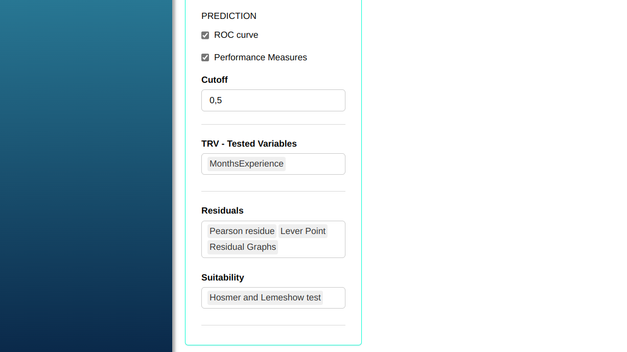
Configuring as shown in the figure below to perform the analysis.

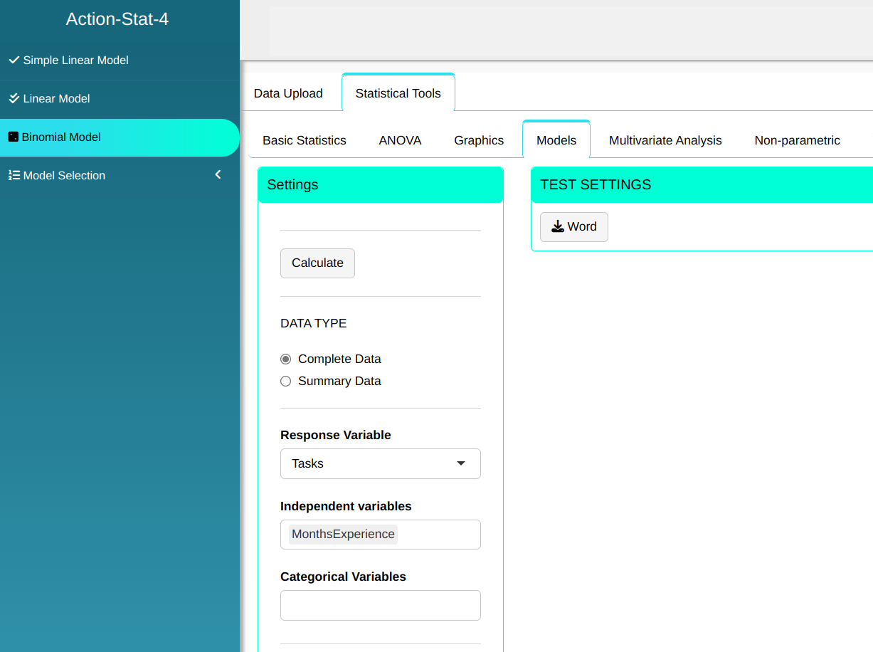
Then click Calculate to get the results. You can also generate the analyses and download them in Word format.

The results are:

Estimated Coefficients Table

	Estimate	Standard Deviation	Wald Test	P-Value	Lower Limit	Upper Limit
Intercept	-3.0596959	1.25934986	-2.429584	0.0151	-5.52797622	-0.5914155
MonthsExperirnce	0.1614859	0.06498001	2.485163	0.0129	0.03412744	0.2888444

---

Covariance Matrix

	(Intercept)	MonthsExperience
(Intercept)	1.5859621	-0.075402604
MonthsExperience	-0.0754026	0.004222402

---

General Information

Information	Value
Fisher Scoring Interation	4
Null Deviance	34.296 with 24 Degrees the Freedom
Residual Deviance	25.425 with 23 Degrees the Freedom
AIC	29.4245740804509
Dispersion Parameter	1

---

Resultado da análise

	Real	V2
Predito	Tasks=0	Tasks=1
Tasks=0	13	6
Tasks=1	1	5

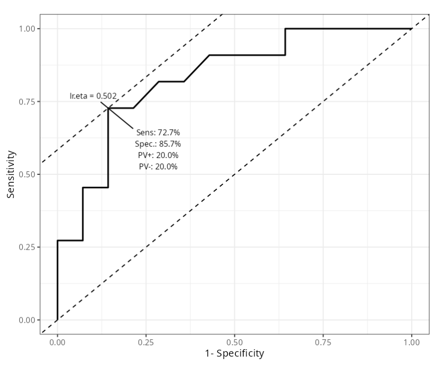
Summary (Performance)

	Percentage (%)
Sensitivity	45.45455
Specificity	92.85714
PPV	83.33333
NPV	68.42105
Accuracy	72.00000

Odds-Ratio Table

Variable	Category	Odds Ratio	Lower Limit	Upper Limit
MonthsExperience		1.1752559100685	1.03471646443219	1.3348840012021

---

Intervalo de Previsão

	MonthsExperience	Adjusted Probability	LL	UL	Standard Deviation
1	14	0.31026237	0.079658965	0.5408658	0.11765696
2	29	0.83526292	0.599589805	1.0709360	0.12024360
3	6	0.10999616	-0.065139980	0.2851323	0.08935681
4	25	0.72660237	0.464020009	0.9891847	0.13397306
5	18	0.46183704	0.223425450	0.7002486	0.12164080
6	4	0.08213002	-0.069291566	0.2335516	0.07725733
7	12	0.24566554	0.020497984	0.4708331	0.11488352
8	22	0.62081158	0.363141740	0.8784814	0.13146662
9	30	0.85629862	0.632385431	1.0802118	0.11424352
10	11	0.21698039	-0.003406564	0.4373674	0.11244439
11	5	0.09515416	-0.068239496	0.2585478	0.08336564
12	20	0.54240353	0.294917361	0.7898897	0.12627078
13	13	0.27680234	0.048333968	0.5052707	0.11656764
14	9	0.16709980	-0.038978483	0.3731781	0.10514391
15	32	0.89166416	0.694547616	1.0887807	0.10057152
16	24	0.69337941	0.430252386	0.9565064	0.13425095
17	19	0.50213414	0.259630105	0.7446382	0.12372882
18	28	0.81182461	0.566052911	1.0575963	0.12539603
19	8	0.14581508	-0.050963101	0.3425933	0.10039887

---

Prediction Interval

	MonthsExperieence	Adjusted Probability	LL	UL	Stadard Deviation
1	14	0.31026237	0.079658965	0.5408658	0.11765696
2	29	0.83526292	0.599589805	1.0709360	0.12024360
3	6	0.10999616	-0.065139980	0.2851323	0.08935681
4	25	0.72660237	0.464020009	0.9891847	0.13397306
5	18	0.46183704	0.223425450	0.7002486	0.12164080
6	4	0.08213002	-0.069291566	0.2335516	0.07725733
7	18	0.46183704	0.223425450	0.7002486	0.12164080
8	12	0.24566554	0.020497984	0.4708331	0.11488352
9	22	0.62081158	0.363141740	0.8784814	0.13146662
10	6	0.10999616	-0.065139980	0.2851323	0.08935681
11	30	0.85629862	0.632385431	1.0802118	0.11424352
12	11	0.21698039	-0.003406564	0.4373674	0.11244439
13	30	0.85629862	0.632385431	1.0802118	0.11424352
14	5	0.09515416	-0.068239496	0.2585478	0.08336564
15	20	0.54240353	0.294917361	0.7898897	0.12627078
16	13	0.27680234	0.048333968	0.5052707	0.11656764
17	9	0.16709980	-0.038978483	0.3731781	0.10514391
18	32	0.89166416	0.694547616	1.0887807	0.10057152
19	24	0.69337941	0.430252386	0.9565064	0.13425095
20	13	0.27680234	0.048333968	0.5052707	0.11656764
21	19	0.50213414	0.259630105	0.7446382	0.12372882
22	4	0.08213002	-0.069291566	0.2335516	0.07725733
23	28	0.81182461	0.566052911	1.0575963	0.12539603
24	22	0.62081158	0.363141740	0.8784814	0.13146662
25	8	0.14581508	-0.050963101	0.3425933	0.10039887

Likelihood-Ratio Test (LRT)

Tested Variables	Test Statisti	Degrees of Freedom	P-Value
MonthsExperience	8.871916	1	0.002895911

---

Hormer and Lemeshow Test

	Test Statistic	Degrees of Freedom	P-Value	Number of groups
tabHosmer	0.8636609	1	0.3527162	3
X	0.1032996	2	0.9496614	4
X.1	2.1663561	3	0.5386055	5
X.2	1.6652041	4	0.7970282	6
X.3	3.4095112	5	0.6371218	7
X.4	3.1422227	6	0.7907964	8
X.5	6.4255004	7	0.4910340	9
X.6	6.5599688	8	0.5847638	10

---

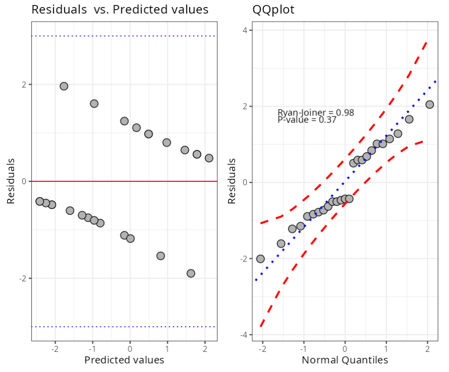
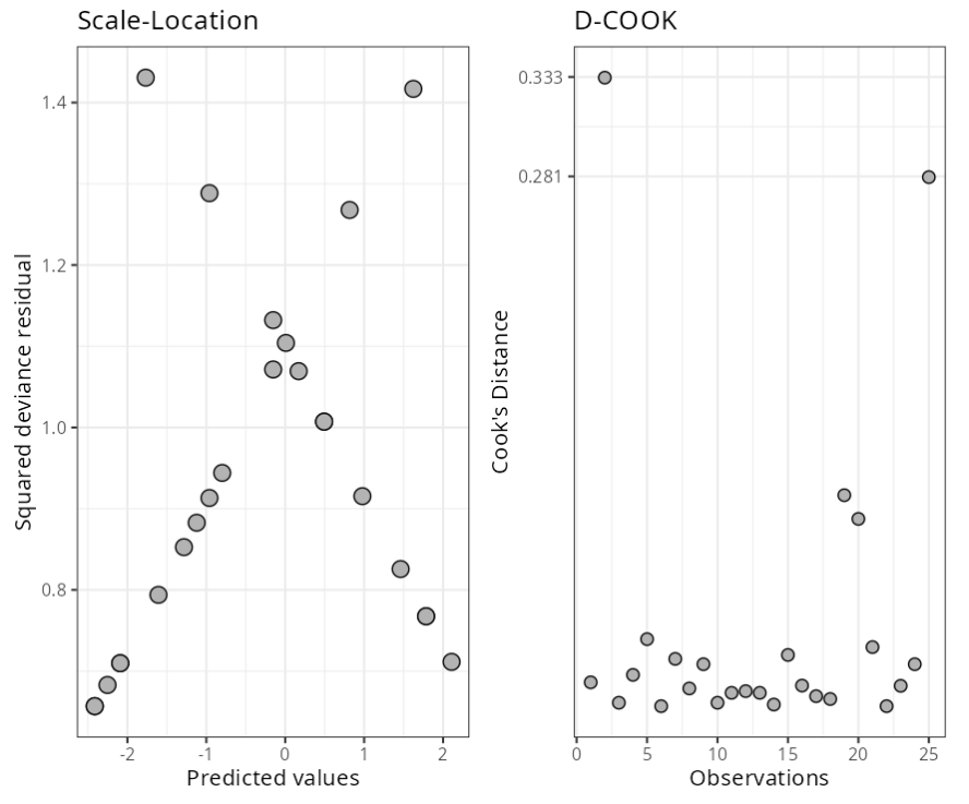
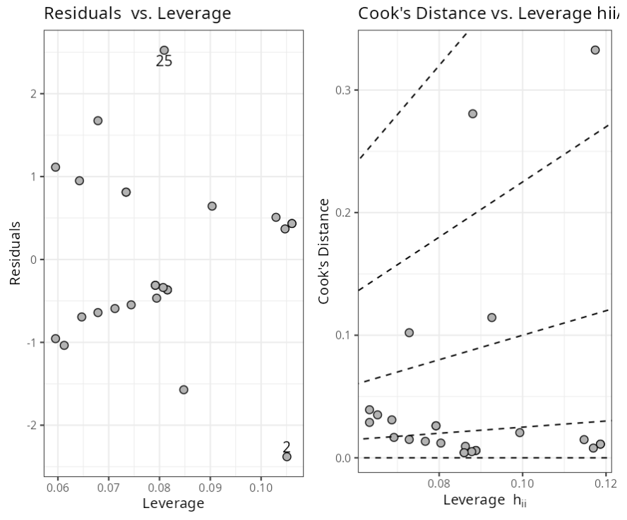
Residual Table

	Deviance Residual	Pearson Residual	Leverage	Cook’s Distance
1	-0.8912168	-0.6934965	0.06468785	0.016631244
2	-2.0075616	-2.3802536	0.10507761	0.332614571
3	-0.5037418	-0.3668326	0.08156202	0.005975083
4	0.8379723	0.6431504	0.09035322	0.020543100
5	1.2817536	1.1131167	0.05953276	0.039216040
6	-0.4314357	-0.3117255	0.07917694	0.004177699
7	-1.1478806	-0.9552469	0.05953276	0.028881095
8	-0.7791504	-0.5921530	0.07122100	0.013444157
9	1.0143989	0.8119069	0.07342029	0.026116551
10	-0.5037418	-0.3668326	0.08156202	0.005975083
11	0.5891404	0.4332766	0.10606643	0.011137127
12	-0.7269990	-0.5471630	0.07441893	0.012035729
13	0.5891404	0.4332766	0.10606643	0.011137127
14	-0.4664129	-0.3382224	0.08071868	0.005022274
15	1.1434517	0.9495059	0.06423926	0.030945750
16	-0.8338729	-0.6407963	0.06787813	0.014950895
17	-0.6302671	-0.4668354	0.07943296	0.009402490
18	0.5061151	0.3683859	0.10470752	0.007935766
19	-1.6072596	-1.5718845	0.08477399	0.114431488
20	1.6601125	1.6741998	0.06787813	0.102056745
21	-1.2189489	-1.0365150	0.06123640	0.035040847
22	-0.4314357	-0.3117255	0.07917694	0.004177699
23	0.6817493	0.5083200	0.10293029	0.014823864
24	1.0143989	0.8119069	0.07342029	0.026116551
25	2.0469291	2.5246445	0.08092914	0.280625042

---