2. Linear Model
The linear model is used to analyze the relationship between two or more variables.
Example 1:
The gain of a transistor is the difference between the emitter and the collector. The Gain variable (in hFE) can be controlled in the ion deposition process through the variables Emission time (in minutes) and Ion dose ($ \times 10^{14} $) variables. The data is shown in Table 1. Our aim is to evaluate the linear relationship between transistor gain and the covariates Emission Time and Ion Dose.
| Time | Dose | Gain |
|---|---|---|
| 195 | 4 | 1004 |
| 255 | 4 | 1636 |
| 195 | 4.6 | 852 |
| 255 | 4.6 | 1506 |
| 225 | 4.2 | 1272 |
| 225 | 4.1 | 1270 |
| 225 | 4.6 | 1269 |
| 195 | 4.3 | 903 |
| 255 | 4.3 | 1555 |
| 225 | 4 | 1260 |
| 225 | 4.7 | 1146 |
| 225 | 4.3 | 1276 |
| 225 | 4.72 | 1225 |
| 230 | 4.3 | 1321 |
We will upload the data to the system.
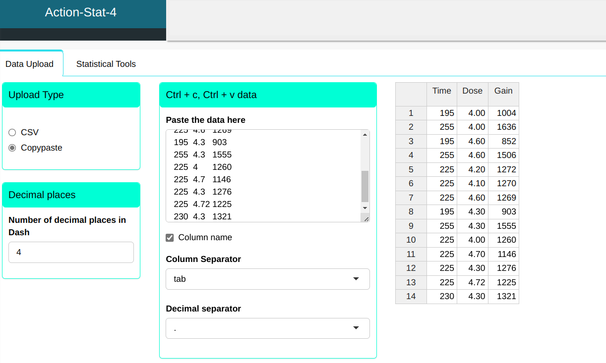
Configuring as shown in the figure below to perform the analysis.
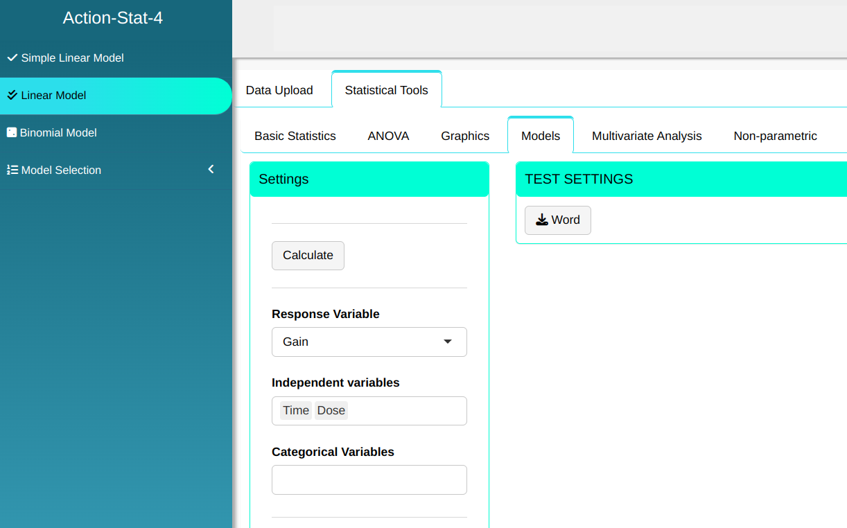
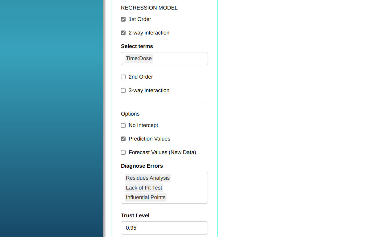

Then click Calculate to get the results. You can also generate the analyses and download them in Word format.

The results are:
ANOVA Table
| D.F. | Sum of Squares | Mean Square | F Stat. | P-value | |
|---|---|---|---|---|---|
| Time | 1 | 630967.86 | 630967.865 | 474.40781465 | 0 |
| Dose | 1 | 20998.23 | 20998.234 | 15.78800898 | 0.0026287995665368 |
| Time:Dose | 1 | 121.00 | 121.000 | 0.09097665 | 0.7691183430521420 |
| Residuals | 10 | 13300.12 | 1330.012 |
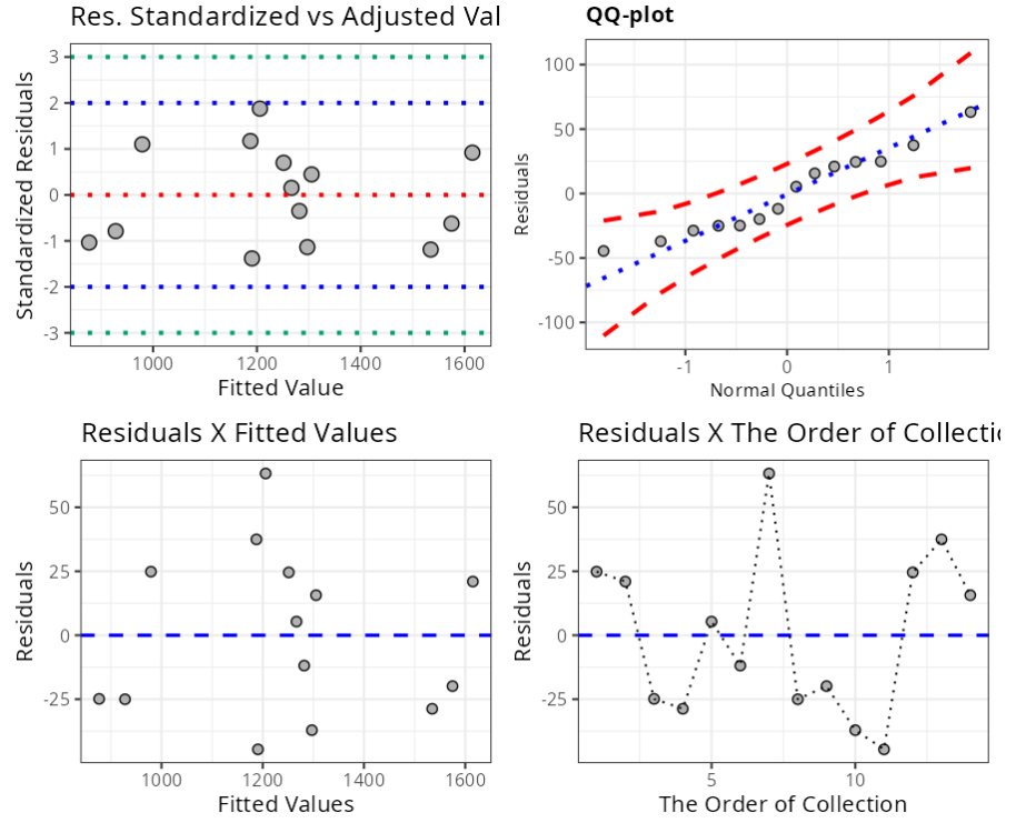
Expĺoratory Analysis (residues)
| Minimum | 1Q | Median | Mean | 3Q | Maximum |
|---|---|---|---|---|---|
| -44.58414 | -25.94015 | -3.266019 | 0 | 24.62883 | 63.20097 |
Coefficients
| Estimate | Standard Deviation | T Stat. | P-value | |
|---|---|---|---|---|
| Intercept | 71.1733231 | 1,970.46088 | 0.03612014 | 0.971897 |
| Time | 8.1533801 | 8.726180 | 0.93435849 | 0.372131 |
| Dose | -289.648874 | 457.471922 | -0.6331511 | 0.540843 |
| Time:Dose | 0.6111111 | 2.026074 | 0.30162337 | 0.769118 |
Descriptive measure for Goodness-of-Fit
| Standard deviation of residuals | Degrees of Freedom | R^2 | Adjusted R^2 |
|---|---|---|---|
| 36.46932 | 10 | 0.980011 | 0.9740149 |
Confidence Interval for the parameters
| 2.5 % | 97.5 % | |
|---|---|---|
| Intercept | -4319.287130 | 4461.633776 |
| Time | -11.289760 | 27.596520 |
| Dose | -1308.959837 | 729.662088 |
| Time:Dose | -3.903262 | 5.125484 |
Prediction Interval
| Gain | Time | Dose | Fitted Value | Lower Limit | Upper Limit | Standard Deviation |
|---|---|---|---|---|---|---|
| 1,004 | 195 | 4.00 | 979.1536 | 915.3027 | 1043.0045 | 28.656620 |
| 1636 | 255 | 4.00 | 1615.0231 | 1551.6616 | 1678.3846 | 28.436947 |
| 852 | 195 | 4.60 | 876.8643 | 815.6809 | 938.0477 | 27.459417 |
| 1506 | 255 | 4.60 | 1534.7338 | 1473.9136 | 1595.5539 | 27.296389 |
| 1272 | 225 | 4.20 | 1266.6586 | 1241.9861 | 1291.3311 | 11.073149 |
| 1270 | 225 | 4.10 | 1281.8735 | 1252.1883 | 1311.5586 | 13.322842 |
| 1269 | 225 | 4.60 | 1205.799 | 1174.5787 | 1237.0194 | 14.011854 |
| 903 | 195 | 4.30 | 928.0090 | 887.9554 | 968.0625 | 17.976226 |
| 1555 | 255 | 4.30 | 1574.8784 | 1535.4958 | 1614.2611 | 17.675135 |
| 1260 | 225 | 4.00 | 1297.0883 | 1261.0430 | 1333.1337 | 16.177353 |
| 1146 | 225 | 4.70 | 1190.5841 | 1152.7665 | 1228.4018 | 16.972751 |
| 1276 | 225 | 4.30 | 1251.4437 | 1229.4927 | 1273.3947 | 9.851714 |
| 1225 | 225 | 4.72 | 1187.5412 | 1148.3144 | 1226.7679 | 17.605162 |
| 1321 | 230 | 4.30 | 1305.3495 | 1282.8141 | 1327.8849 | 10.113995 |
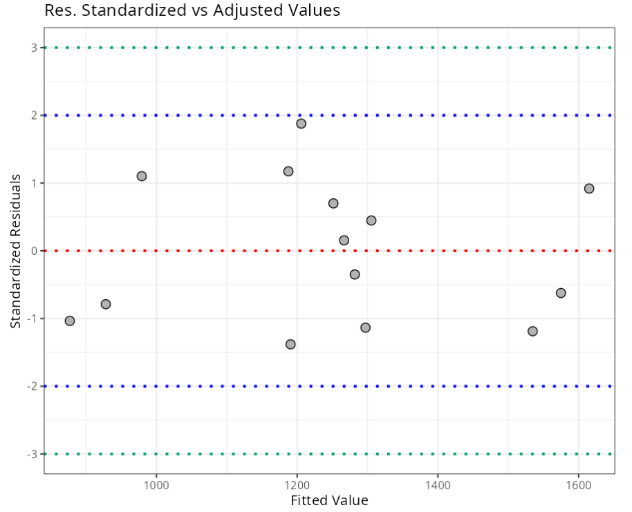
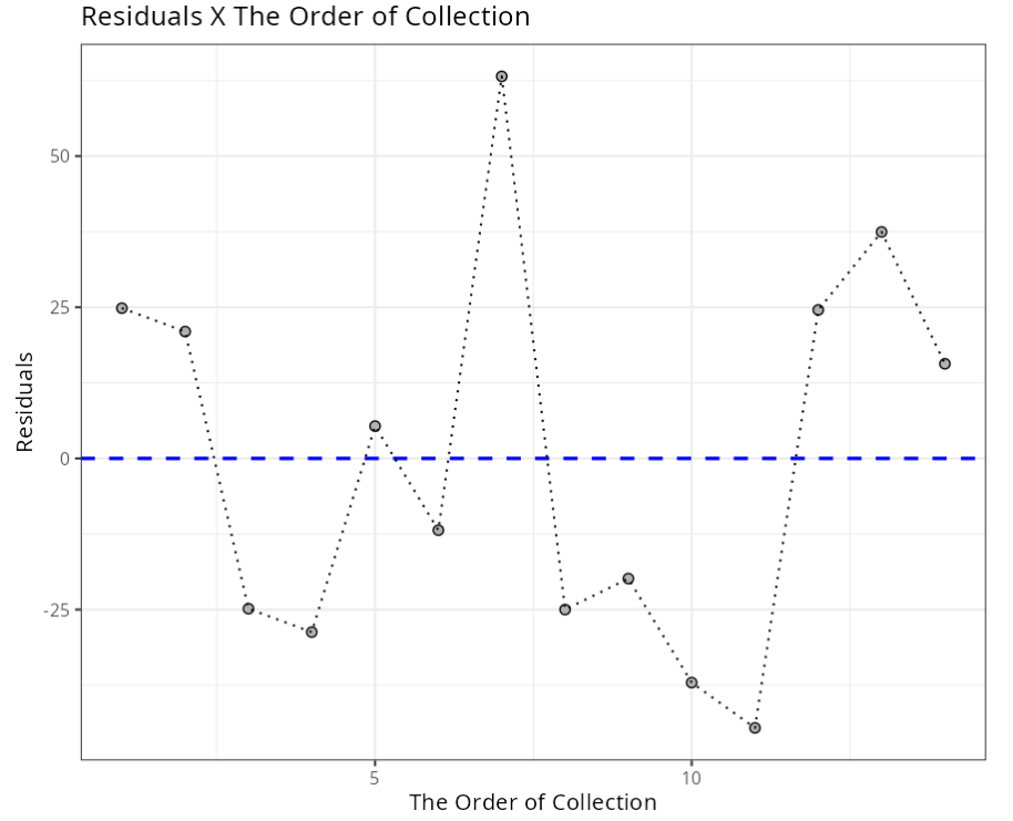
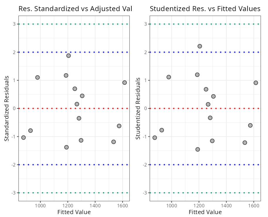
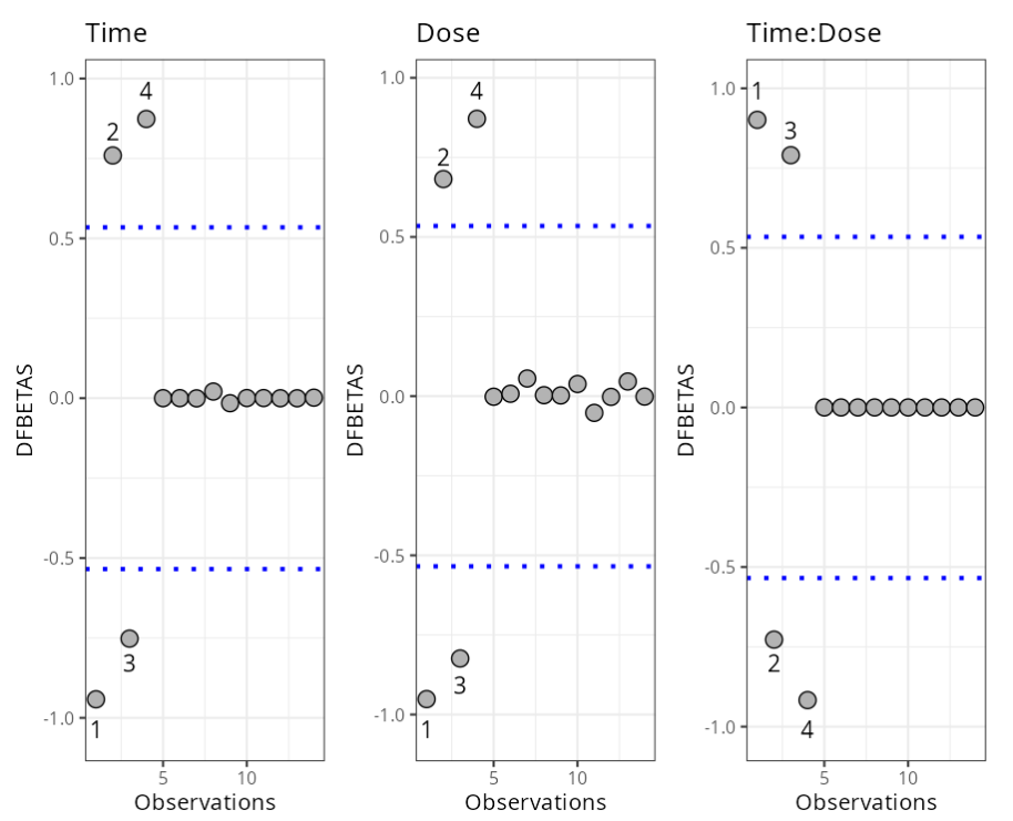
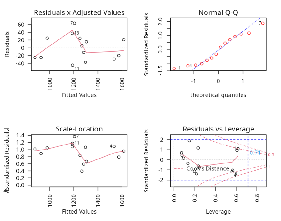
Summary of Residuals Analysis
| N.Obs | Time | Dose | Residuals | Studentized Residuals | Standardized Residuals | Leverage | DFFITS | DFBETA | D-COOK |
|---|---|---|---|---|---|---|---|---|---|
| 1 | 195 | 4.00 | 24.846387 | 1.1147927 | 1.1015027 | 0.61743967 | 1.41625490 | -0.94199418165 | 0.4895597961 |
| 2 | 255 | 4.00 | 20.976913 | 0.9108462 | 0.9187053 | 0.60800973 | 1.13439076 | 0.75939078067 | 0.3272862194 |
| 3 | 195 | 4.60 | -24.864288 | -1.0402662 | -1.0360193 | 0.56692711 | -1.19022098 | -0.75218753067 | 0.3512706755 |
| 4 | 255 | 4.60 | -28.733762 | -1.2162085 | -1.1880774 | 0.56021533 | -1.37266797 | 0.87352758220 | 0.4495152217 |
| 5 | 225 | 4.20 | 5.341425 | 0.1460048 | 0.1537206 | 0.09219065 | 0.04652787 | -0.00004549144 | 0.0005999243 |
| 6 | 225 | 4.10 | -11.873462 | -0.3338476 | -0.3497473 | 0.13345608 | -0.13101533 | 0.00011212495 | 0.0047097360 |
| 7 | 225 | 4.60 | 63.200975 | 2.2127130 | 1.8770621 | 0.14761681 | 0.92082173 | -0.00056023133 | 0.1525450911 |
| 8 | 195 | 4.30 | -25.008951 | -0.7720700 | -0.7881510 | 0.24296384 | -0.43739033 | 0.02076432661 | 0.0498406795 |
| 9 | 255 | 4.30 | -19.878424 | -0.6029964 | -0.6231508 | 0.23489299 | -0.33410935 | -0.01574389071 | 0.0298039755 |
| 10 | 225 | 4.00 | -37.088350 | -1.1532997 | -1.1347232 | 0.19677029 | -0.57082381 | 0.00042262343 | 0.0788568872 |
| 11 | 225 | 4.70 | -44.584138 | -1.4566189 | -1.3812096 | 0.21659532 | -0.76590938 | 0.00035872582 | 0.1318627421 |
| 12 | 225 | 4.30 | 24.556312 | 0.6802984 | 0.6993418 | 0.07297401 | 0.19086997 | -0.00019860744 | 0.0096248792 |
| 13 | 225 | 4.72 | 37.458840 | 1.1981057 | 1.1728416 | 0.23303688 | 0.66041999 | -0.00029388986 | 0.1044886083 |
| 14 | 230 | 4.30 | 15.650523 | 0.4280325 | 0.4466624 | 0.07691128 | 0.12355207 | 0.00159139594 | 0.0041557123 |
Criterion
| Diagnostic | Formula | Value |
|---|---|---|
| hii (Leverage) | (2*(p+1))/n | 0.57 |
| DFFITS | 2* Square root ((p+1)/n) | 1.1 |
| DCOOK | 4/n | 0.2857143 |
| DFBETA | 2/Square root(n) | 0.53 |
| Standardized Residuals | (-3,3) | 3 |
| Studentized Residuals | (-3,3) | 3 |
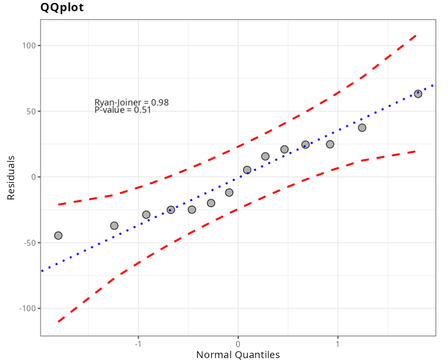
Normality Test
| Statistics | P-value | |
|---|---|---|
| Anderson-Darling | 0.3592592 | 0.3978779 |
| Shapiro-Wilk | 0.9453507 | 0.4911092 |
| Kolmogorov-Smirnov | 0.1614289 | 0.4142572 |
| Ryan-Joiner | 0.9761196 | 0.5098 |
Homoscedasticity Test - Breusch Pagan
| Statistics | DF | P-value |
|---|---|---|
| 0.2119295 | 1 | 0.6452593 |
Homoscedasticity Test - Goldfeld Quandt
| Variable | Statistics | DF1 | DF2 | P-value |
|---|---|---|---|---|
| Time | 0.212367391304331 | 2 | 1 | 0.324428433008958 |
| Dose | 1.70140146940424 | 2 | 1 | 0.953159041390766 |
Independence Test - Durbin-Watson
| Statistics | P-value |
|---|---|
| 1.71481 | 0.8201288 |
Lack of Fit Test
| $\qquad \quad$Lack of fit test | ||
| Input data do not contain replicas |
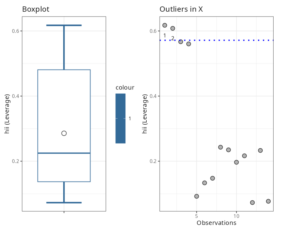
Outliers (X)
| Observations | Leverage | Criterin |
|---|---|---|
| 1 | 0.6174397 | 0.5714286 |
| 2 | 0.6080097 | 0.5714286 |
Outliers (atypical points)
| Observation | T-Value | P-Value | P-Value Bonferroni |
|---|---|---|---|
| 7 | 2.212713 | 0.05420479 | 0.758867 |
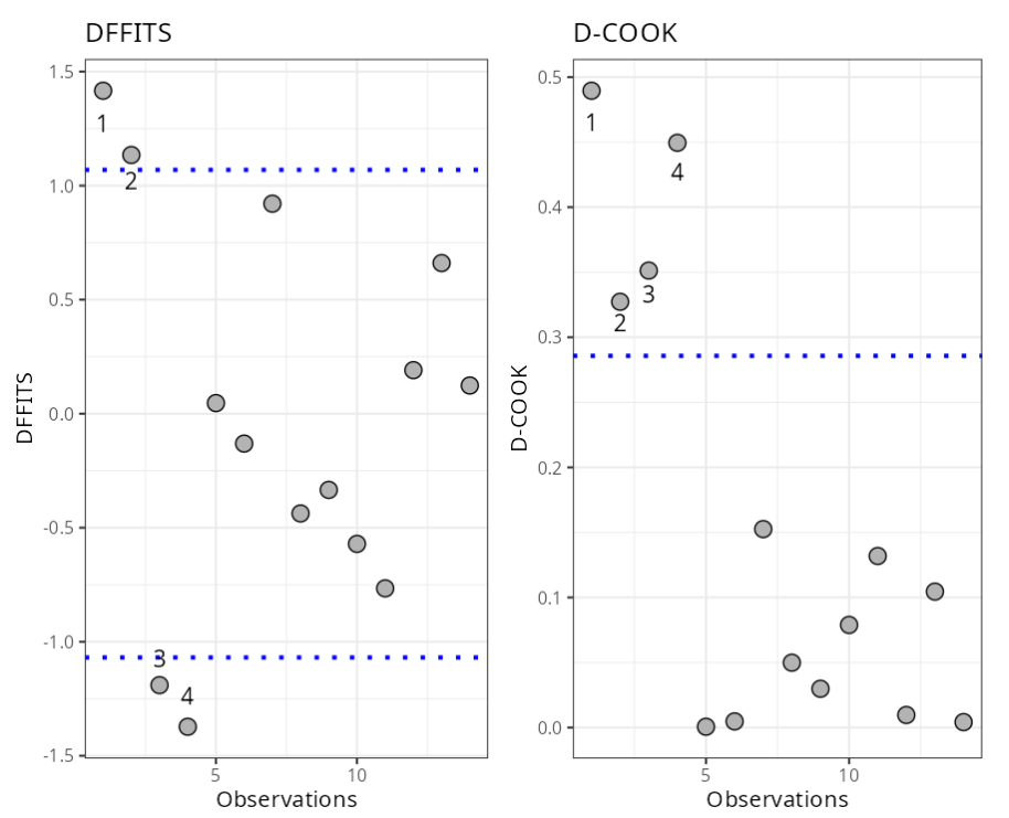
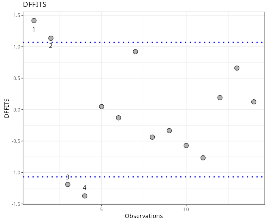
Influential Point
| Observations | DFFITS | Criterion |
|---|---|---|
| 1 | 1.42 | ± 1.07 |
| 2 | 1.13 | ± 1.07 |
| 3 | -1.19 | ± 1.07 |
| 4 | -1.37 | ± 1.07 |
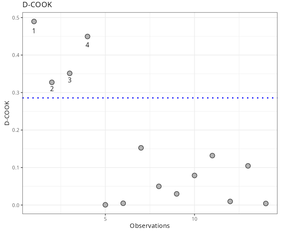
Influential Points
| Observations | DCOOK | Criterio |
|---|---|---|
| 1 | 0.4895598 | 0.2857143 |
| 2 | 0.3272862 | 0.2857143 |
| 3 | 0.3512707 | 0.2857143 |
| 4 | 0.4495152 | 0.2857143 |
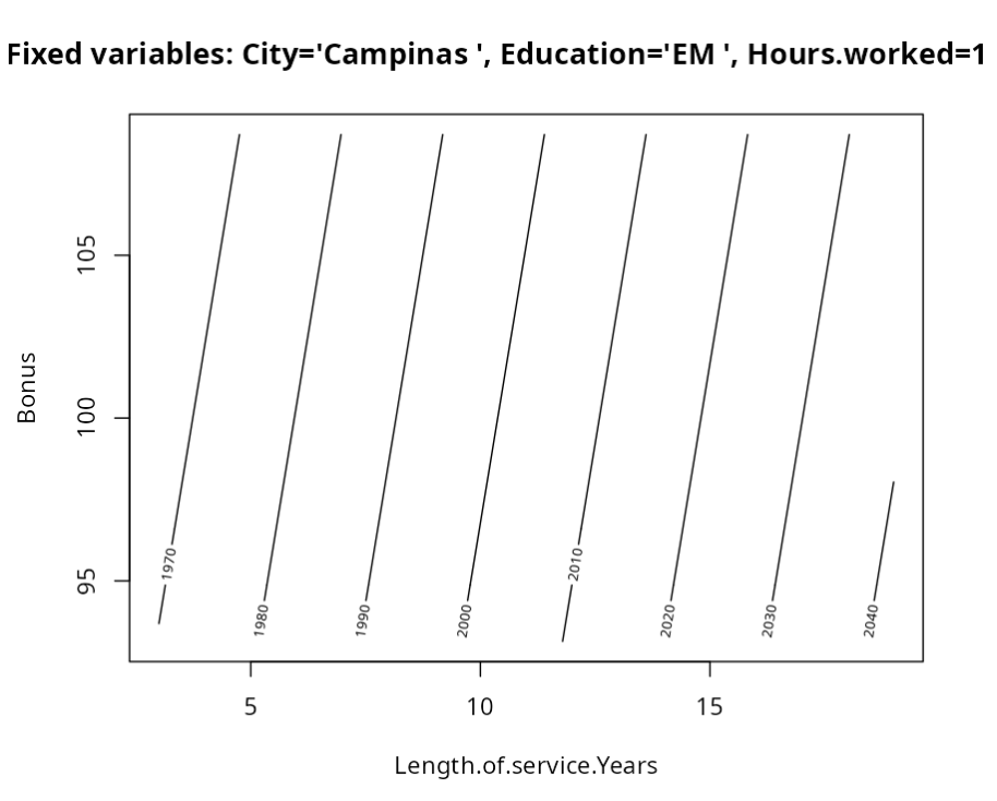
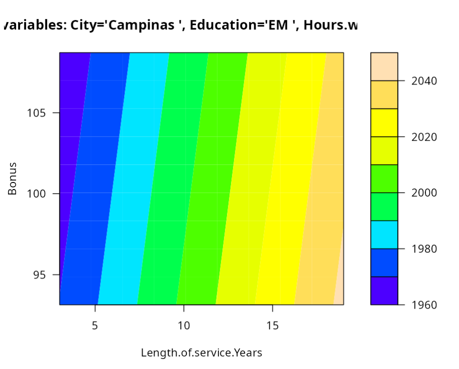
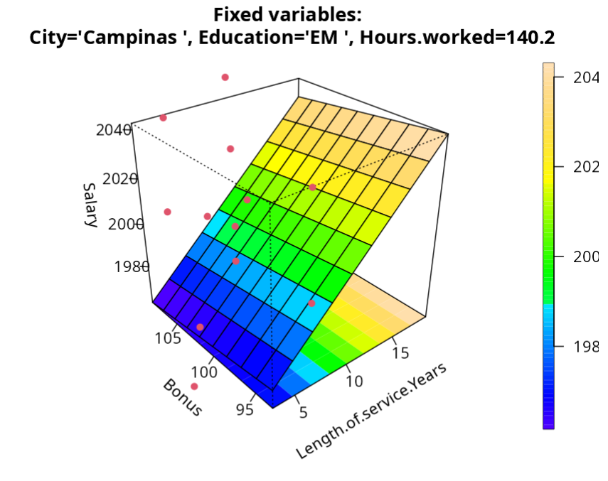
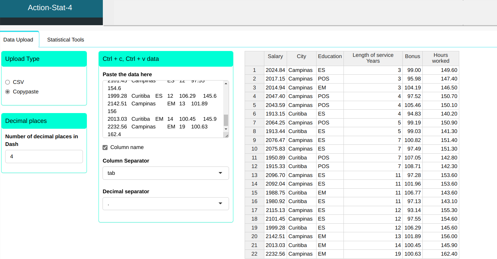
Example 2:
The monthly net salary of employees at a federal university is linearly related to the variables City of employment (Campus the Campinas and Curitiba), Education (Higher Education Completed, Postgraduate Degree Completed or High School Degree Completed), Length of Service at the university, total bonuses in the month and Hours Worked in the month. Data was collected from 22 employees. This data can be analyzed in the table below.
| Salary | City | Education | Length of service years | Bonus | Hours worked |
|---|---|---|---|---|---|
| 2024.84 | Campinas | ES | 3 | 99 | 149.6 |
| 2017.15 | Campinas | POS | 3 | 95.98 | 147.4 |
| 2014.94 | Campinas | EM | 3 | 104.19 | 146.5 |
| 2047.4 | Campinas | POS | 4 | 97.52 | 150.7 |
| 2043.59 | Campinas | POS | 4 | 105.46 | 150.1 |
| 1913.15 | Curitiba | ES | 4 | 94.83 | 140.2 |
| 2064.25 | Campinas | POS | 5 | 99.19 | 150.9 |
| 1913.44 | Curitiba | ES | 5 | 99.03 | 141.3 |
| 2076.47 | Campinas | ES | 7 | 100.82 | 151.4 |
| 2075.83 | Campinas | ES | 7 | 97.49 | 151.3 |
| 1950.89 | Curitiba | POS | 7 | 107.05 | 142.8 |
| 1915.33 | Curitiba | POS | 7 | 108.71 | 142.3 |
| 2096.7 | Campinas | ES | 11 | 97.28 | 153.6 |
| 2092.04 | Campinas | ES | 11 | 101.96 | 153.6 |
| 1988.75 | Curitiba | EM | 11 | 106.77 | 143.6 |
| 1980.92 | Curitiba | ES | 11 | 97.13 | 143.1 |
| 2115.13 | Campinas | ES | 12 | 93.14 | 155.3 |
| 2101.45 | Campinas | ES | 12 | 97.55 | 154.6 |
| 1999.28 | Curitiba | ES | 12 | 106.29 | 145.6 |
| 2142.51 | Campinas | EM | 13 | 101.89 | 156 |
| 2013.03 | Curitiba | EM | 14 | 100.45 | 145.9 |
| 2232.56 | Campinas | EM | 19 | 100.63 | 162.4 |
We will upload the data to the system.
Configuring as shown in the figure below to perform the analysis.
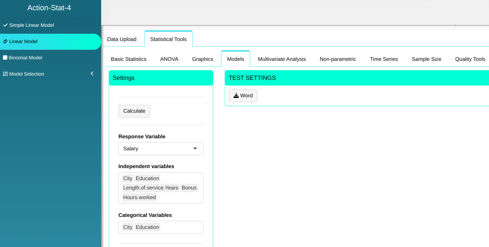
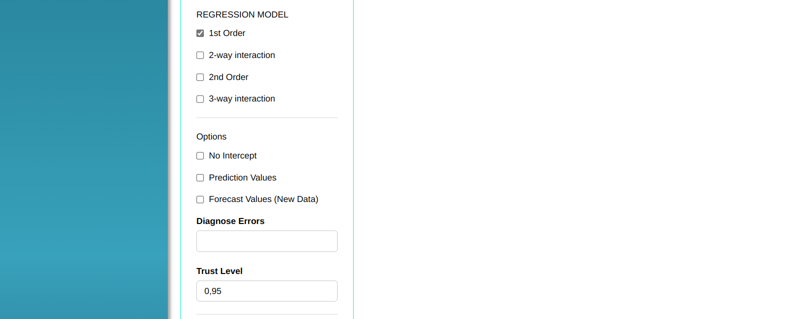


Then click Calculate to get the results. You can also generate the analyses and download them in Word format.
The results are:
ANOVA Table
| D.F. | Sum of Squares | Mean Square | F Stat. | P-Value | |
|---|---|---|---|---|---|
| City | 1 | 76304.3862 | 76304.3862 | 587.6809 | 0.0000 |
| Education | 2 | 17610.2829 | 8805.1414 | 67.8154 | 0.0000 |
| Length.of.service.Years | 1 | 34129.9036 | 34129.9036 | 262.8616 | 0.0000 |
| Bonus | 1 | 71.7808 | 71.7808 | 0.5528 | 0.4686 |
| Hours.worked | 1 | 1445.4002 | 1445.4002 | 11.1322 | 0.0045 |
| Residuals | 15 | 1947.5974 | 129.8398 |
Exploratory Analysis (residues)
| Minimum | 1Q | Median | Mean | 3Q | Maximum |
|---|---|---|---|---|---|
| -23.2602 | -6.455 | 0.1493 | 0 | 8.1092 | 13.7546 |
Coefficients
| Estimate | Standard Deviation | T Stat. | P-value | |
|---|---|---|---|---|
| Intercept | 814.3743 | 377.5276 | 2.1571 | 0.0476 |
| CityCuritiba | -45.6785 | 25.5988 | -1.7844 | 0.0946 |
| EducationES | -16.1322 | 7.2616 | -2.2216 | 0.0421 |
| EducationPOS | -13.7281 | 9.1100 | -1.5069 | 0.1526 |
| Length.of.service.Years | 4.5184 | 2.1280 | 2.1233 | 0.0508 |
| Bonus | -0.5274 | 0.7177 | -0.7348 | 0.4738 |
| Hours.worked | 8.4984 | 2.5471 | 3.3365 | 0.0045 |
Descriptive measure for Goodness-of-Fit
| Standard deviation of residuals | Degrees of Freedom | R^2 | Adjusted R^2 |
|---|---|---|---|
| 11.3947 | 15 | 0.9852 | 0.9793 |
Confidence Interval for the parameters
| 2.5 % | 97.5 % | |
|---|---|---|
| Intercept | 9.6932 | 1619.0554 |
| CityCuritiba | -100.2411 | 8.8841 |
| EducationES | -31.6100 | -0.6545 |
| EducationPOS | -33.1457 | 5.6894 |
| Length.of.service.Years | -0.0172 | 9.0541 |
| Bonu | -2.0570 | 1.0023 |
| Hours.worked | 3.0694 | 13.9274 |