2. Model Selection: Binomial Model
The Binomial regression model is used when the response variable is qualitative with two possible outcomes. This way we can choose the best binomial model fit for a data set.
Example 1:
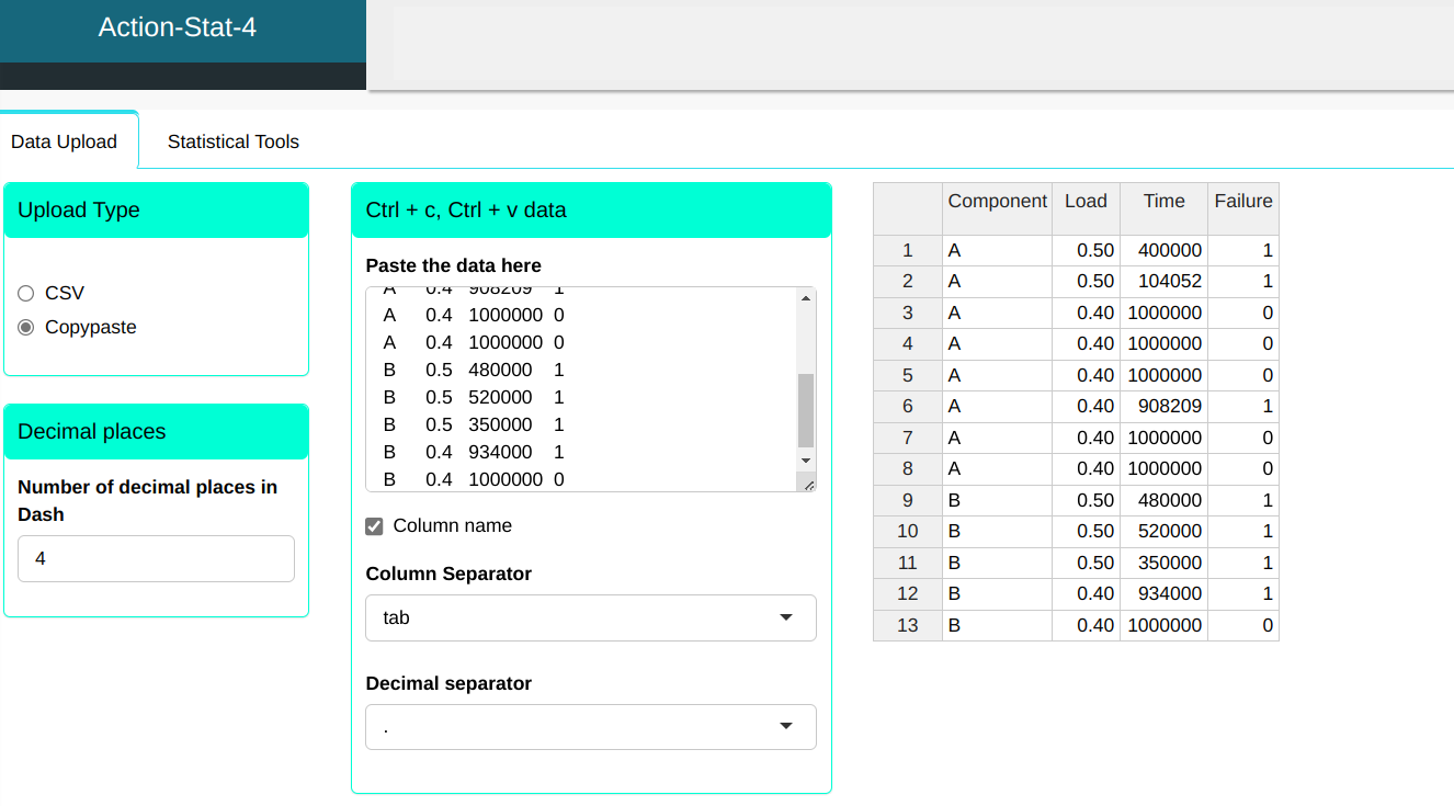
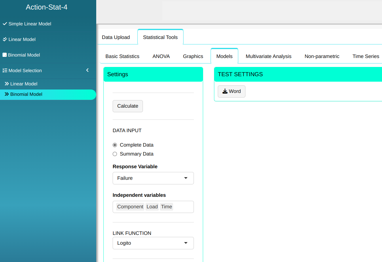
A product engineering team performed a test to evaluate the load that an engine component supports using different materials and time until test failure.
| Component | Load | Time | Failure |
|---|---|---|---|
| A | 0.5 | 400000 | 1 |
| A | 0.5 | 104052 | 1 |
| A | 0.4 | 1000000 | 0 |
| A | 0.4 | 1000000 | 0 |
| A | 0.4 | 1000000 | 0 |
| A | 0.4 | 908209 | 1 |
| A | 0.4 | 1000000 | 0 |
| A | 0.4 | 1000000 | 0 |
| B | 0.5 | 480000 | 1 |
| B | 0.5 | 520000 | 1 |
| B | 0.5 | 350000 | 1 |
| B | 0.4 | 934000 | 1 |
| B | 0.4 | 1000000 | 0 |
We will upload the data to the system.
Configuring as shown in the figure below to perform the analysis.

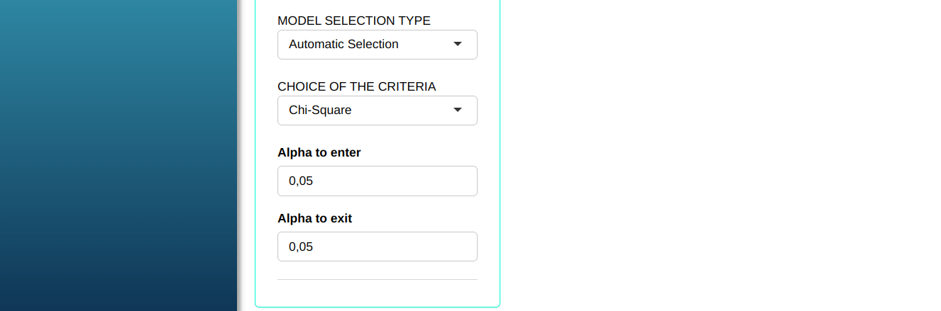
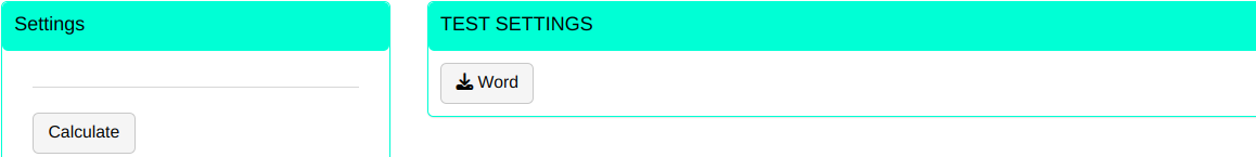
Then click Calculate to get the results. You can also generate the analyses and download them in Word format.
The results are:
Model Selection Table
| Model(Steps) | Variable In | Variable out | LRT | P-Value |
|---|---|---|---|---|
| Model 1 Time | 17.9448 | 2.274015e-05 | ||
| Selected Model | Time |
Deviance Analysis Table
| Variable | D.F. | Deviance | df.Residual | Residual Deviance |
|---|---|---|---|---|
| Intercept | 12 | 17.9448275764889 | ||
| Time | 1 | 17.9448275741547 | 11 | 2.33418928590677e-09 |
Example 2:
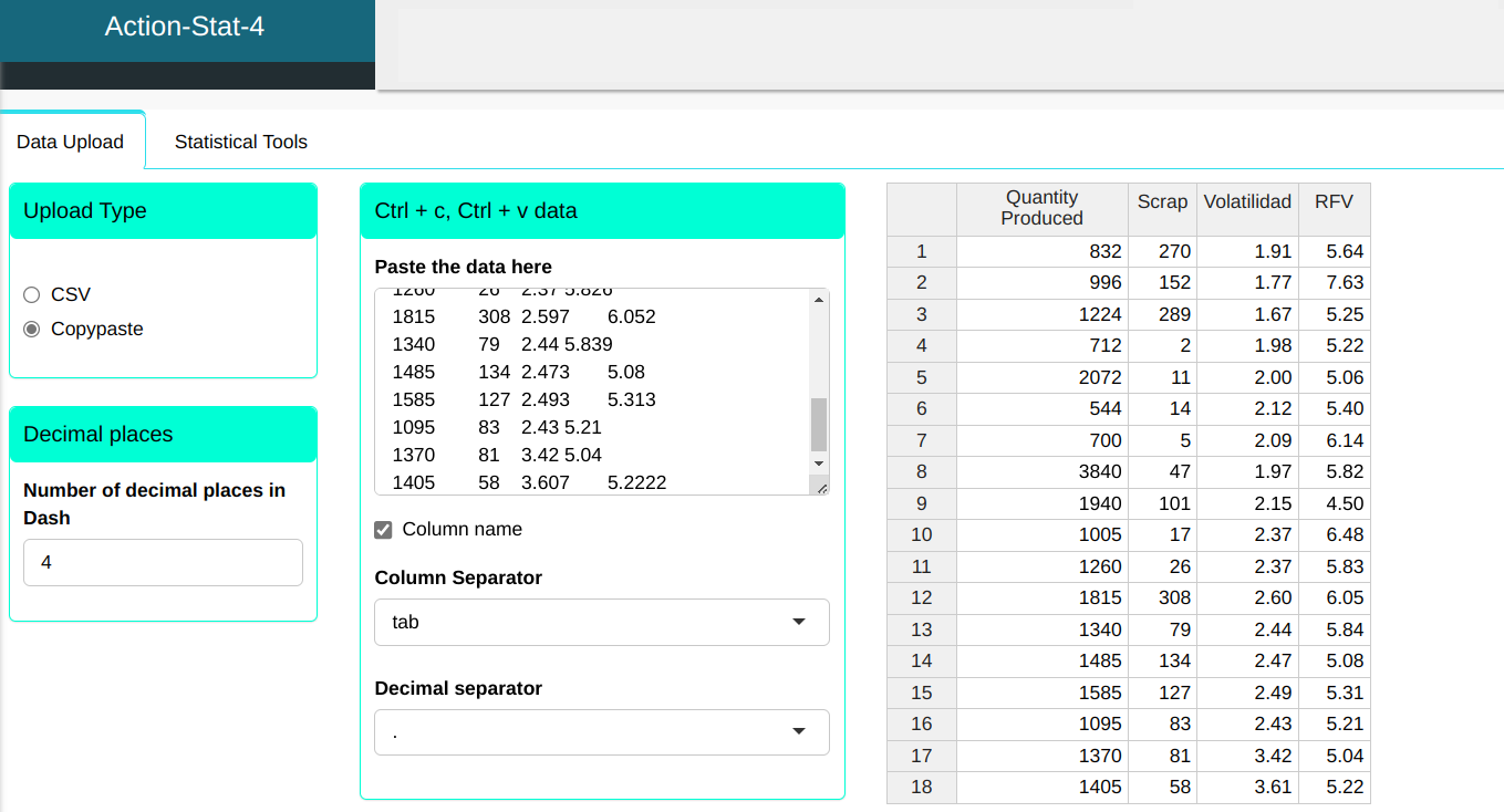
A company manufactures iron parts that are molded in sand molds. Among the parts produced, those with a large amount of embedded sand are considered scrap. The volatility of sand and the RFV (Resistance to Green Fluid) coefficient influence the amount of embedded sand. From the data in the following table, the objective is to evaluate the significance of the variables and the interaction between them, considering the binomial model for response surface.
| Observation | QuantityProduced | Scrap | Volatilidad | RFV |
|---|---|---|---|---|
| 1 | 832 | 270 | 1.906 | 5.642 |
| 2 | 996 | 152 | 1.766 | 7.63 |
| 3 | 1224 | 289 | 1.673 | 5.253 |
| 4 | 712 | 2 | 1.982 | 5.223 |
| 5 | 2072 | 11 | 2 | 5.064 |
| 6 | 544 | 14 | 2.12 | 5.395 |
| 7 | 700 | 5 | 2.085 | 6.138 |
| 8 | 3840 | 47 | 1.97 | 5.82 |
| 9 | 1940 | 101 | 2.15 | 4.498 |
| 10 | 1005 | 17 | 2.37 | 6.478 |
| 11 | 1260 | 26 | 2.37 | 5.826 |
| 12 | 1815 | 308 | 2.597 | 6.052 |
| 13 | 1340 | 79 | 2.44 | 5.839 |
| 14 | 1485 | 134 | 2.473 | 5.08 |
| 15 | 1585 | 127 | 2.493 | 5.313 |
| 16 | 1095 | 83 | 2.43 | 5.21 |
| 17 | 1370 | 81 | 3.42 | 5.04 |
| 18 | 1405 | 58 | 3.607 | 5.2222 |
We will upload the data to the system.
Configuring as shown in the figure below to perform the analysis.
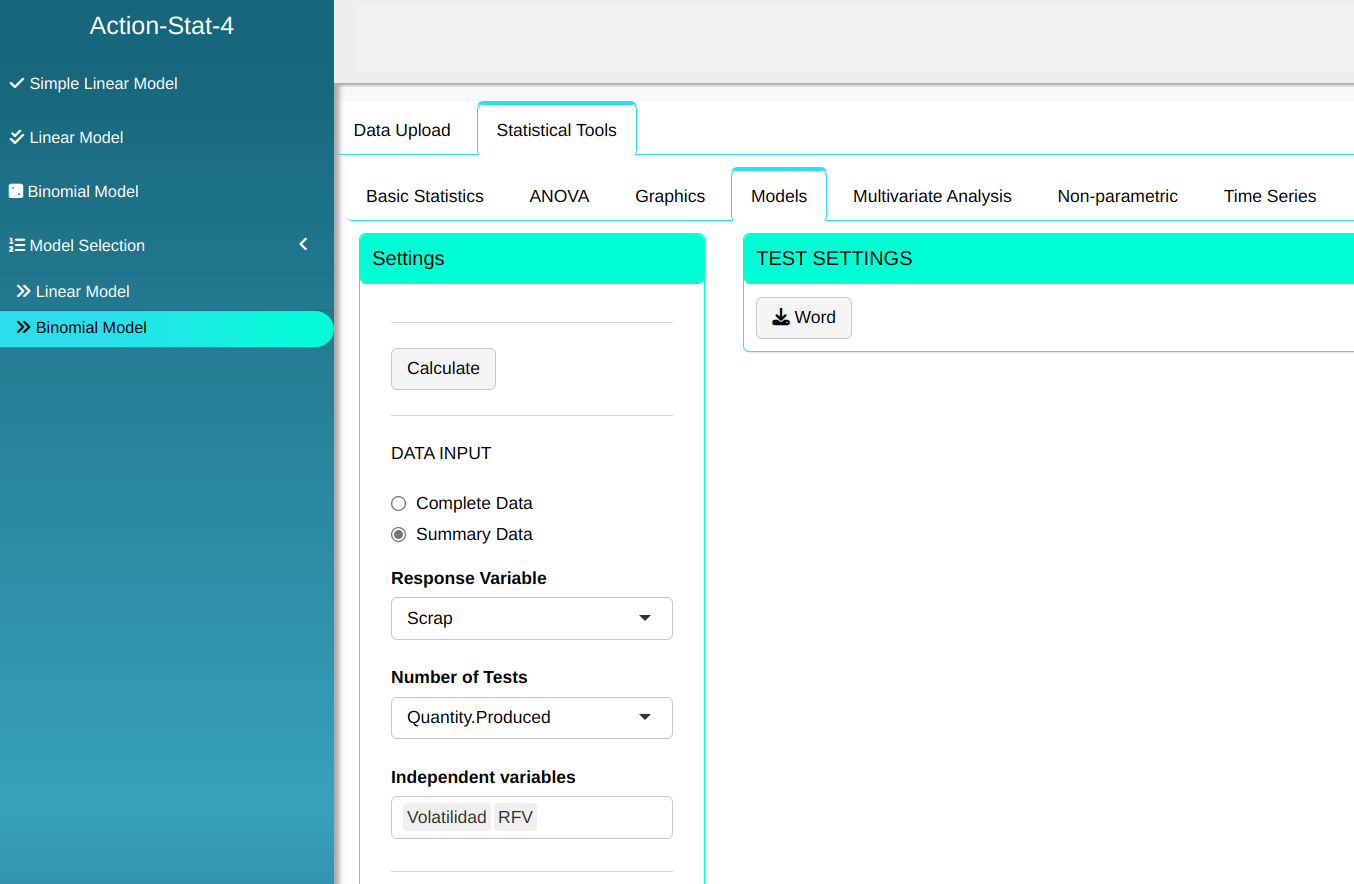
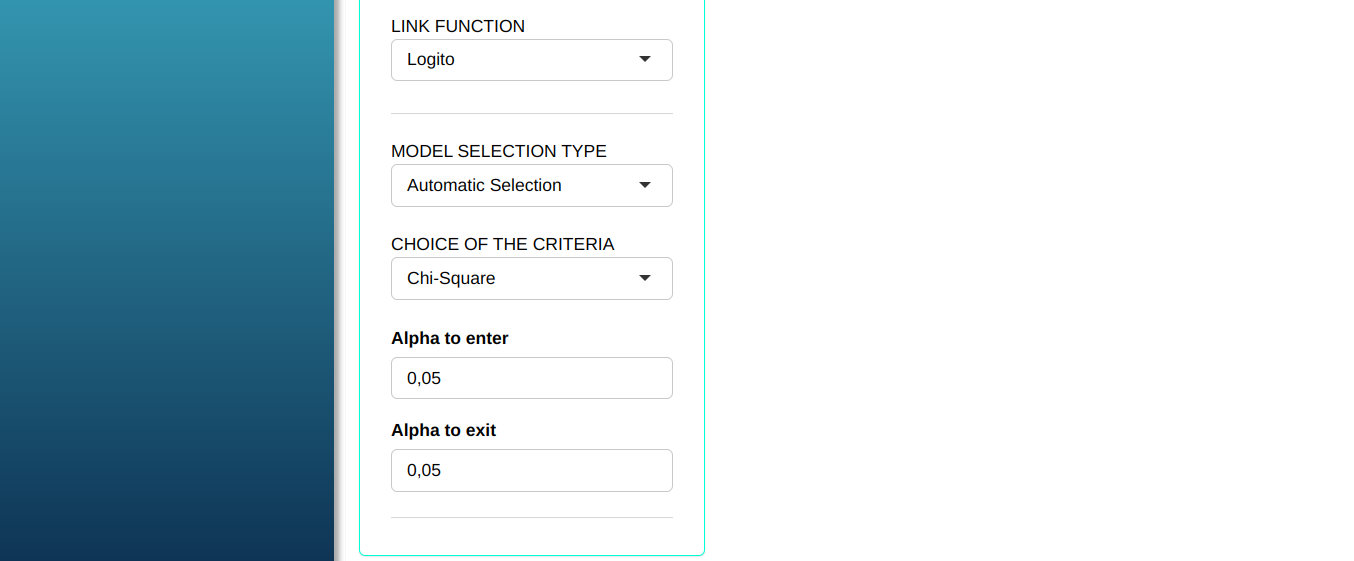
Then click Calculate to get the results. You can also generate the analyses and download them in Word format.
The results are:
Tabela da seleção de modelos
| Modelo(Steps) | Variável Entrou | Variável Saiu | TRV | P-Valor |
|---|---|---|---|---|
| Modelo 1 | RFV. | 48.39399 | 3.486347e-12 | |
| Modelo 2 | Volatilidade | 23.37991 | 1.329596e-06 | |
| Selected Model | RFV. + Volatilidad |
Deviance analysis table
| Variável | G.L. | Deviance | G.L.Residual | Deviance Residual |
|---|---|---|---|---|
| Intercepto | 17 | 1949.04546855248 | ||
| RFV. | 1 | 48.3939919444213 | 16 | 1900.65147660806 |
| Volatilidade | 1 | 23.379914676729 | 15 | 1877.27156193133 |
Example 3:
A product engineering team performed a test to evaluate the load that an engine component supports using different materials and time until test failure.
| Component | Load | Time | Failure |
|---|---|---|---|
| A | 0.5 | 400000 | 1 |
| A | 0.5 | 104052 | 1 |
| A | 0.4 | 1000000 | 0 |
| A | 0.4 | 1000000 | 0 |
| A | 0.4 | 1000000 | 0 |
| A | 0.4 | 908209 | 1 |
| A | 0.4 | 1000000 | 0 |
| A | 0.4 | 1000000 | 0 |
| B | 0.5 | 480000 | 1 |
| B | 0.5 | 520000 | 1 |
| B | 0.5 | 350000 | 1 |
| B | 0.4 | 934000 | 1 |
| B | 0.4 | 1000000 | 0 |
We will upload the data to the system.

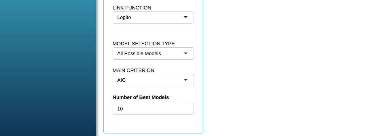
Configuring as shown in the figure below to perform the analysis.

Then click Calculate to get the results. You can also generate the analyses and download them in Word format.
The results are:
Tabela da seleção de modelos
| Models | AIC | BIC | Choose |
|---|---|---|---|
| Time | 2.00000 | 2.564949 | Selected Model |
| Load + Time | 4.00000 | 5.129899 | |
| Component + Time | 4.00000 | 5.129899 | |
| Component + Load + Time | 6.00000 | 7.694848 | |
| Load | 10.99736 | 11.562312 | |
| Component + Load | 12.17932 | 13.309222 | |
| Component | 17.58904 | 17.944828 |
Example 4:
A company manufactures iron parts that are molded in sand molds. Among the parts produced, those with a large amount of embedded sand are considered scrap. The volatility of sand and the RFV (Resistance to Green Fluid) coefficient influence the amount of embedded sand. From the data in the following table, the objective isto assess the significance of the variables and the interaction between them, considering the binomial model for response surface.
| Observation | QuantityProduced | Scrap | Volatilidad | RFV |
|---|---|---|---|---|
| 1 | 832 | 270 | 1.906 | 5.642 |
| 2 | 996 | 152 | 1.766 | 7.63 |
| 3 | 1224 | 289 | 1.673 | 5.253 |
| 4 | 712 | 2 | 1.982 | 5.223 |
| 5 | 2072 | 11 | 2 | 5.064 |
| 6 | 544 | 14 | 2.12 | 5.395 |
| 7 | 700 | 5 | 2.085 | 6.138 |
| 8 | 3840 | 47 | 1.97 | 5.82 |
| 9 | 1940 | 101 | 2.15 | 4.498 |
| 10 | 1005 | 17 | 2.37 | 6.478 |
| 11 | 1260 | 26 | 2.37 | 5.826 |
| 12 | 1815 | 308 | 2.597 | 6.052 |
| 13 | 1340 | 79 | 2.44 | 5.839 |
| 14 | 1485 | 134 | 2.473 | 5.08 |
| 15 | 1585 | 127 | 2.493 | 5.313 |
| 16 | 1095 | 83 | 2.43 | 5.21 |
| 17 | 1370 | 81 | 3.42 | 5.04 |
| 18 | 1405 | 58 | 3.607 | 5.2222 |
We will upload the data to the system.

Configuring as shown in the figure below to perform the analysis.
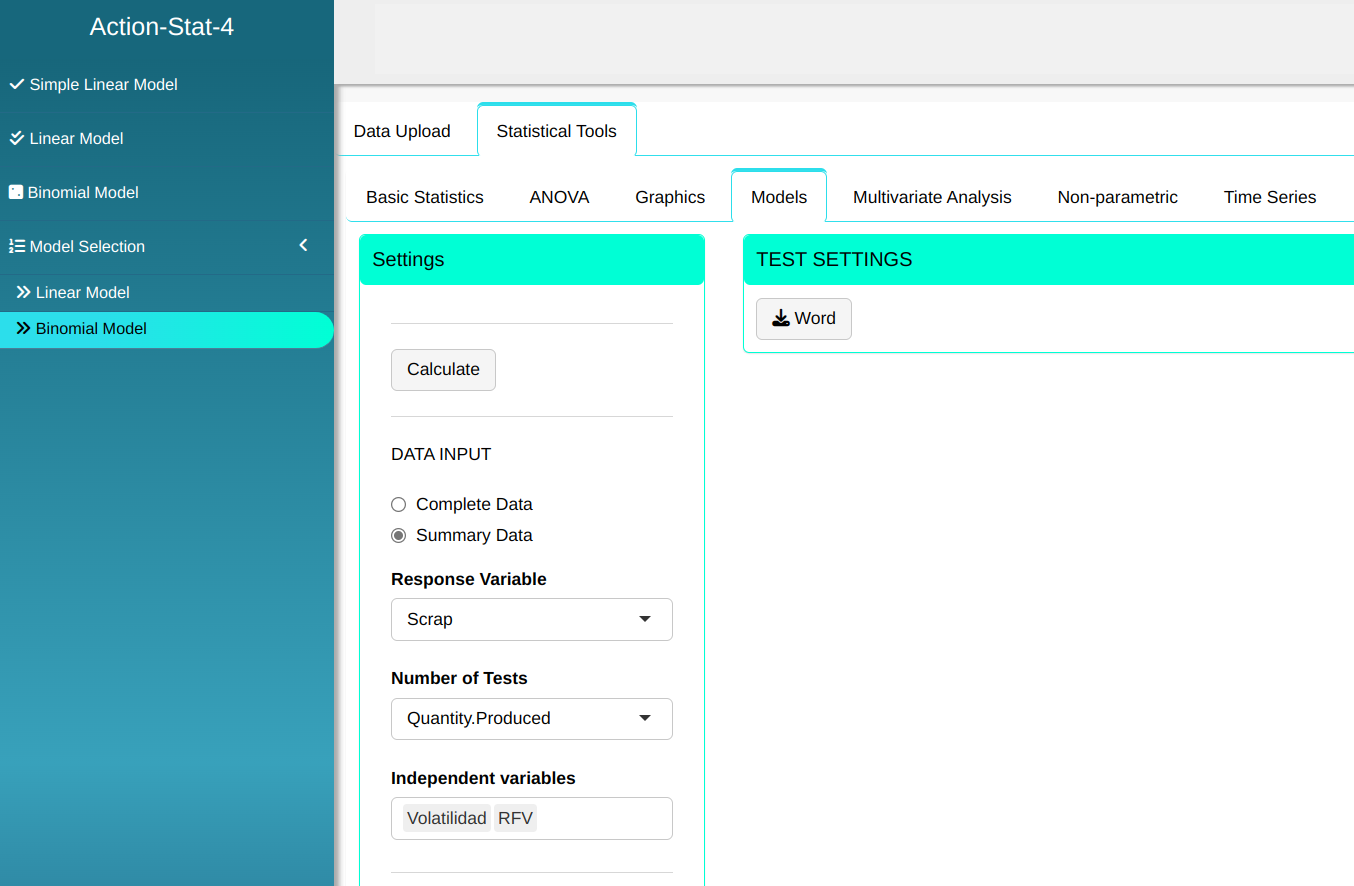
Then click Calculate to get the results. You can also generate the analyses and download them in Word format.
The results are:
Model Selection Table
| Models | AIC | BIC | Choose |
|---|---|---|---|
| Volatilidad + RFV. | 12924.5655 | 12940.8363 | Selected Model |
| RFV. | 12945.9455 | 12954.0808 | |
| Volatilidad | 12953.2066 | 12961.3420 |