3. Rank Test
The Rank Test is the most popular method for comparing survival curves. This test is important when you want to compare a new process with an old one, compare two different products in terms of lifespan or even determine whether two survival curves differ significantly from each other.
Example 1:
A curd cheese producer carries out a durability test on his product, His product is sold at room temperature and without preservatives. The event of interest is the appearance of some fungus on the product. The data is presented below, with the time measured in hours. The + symbol indicates censorship.
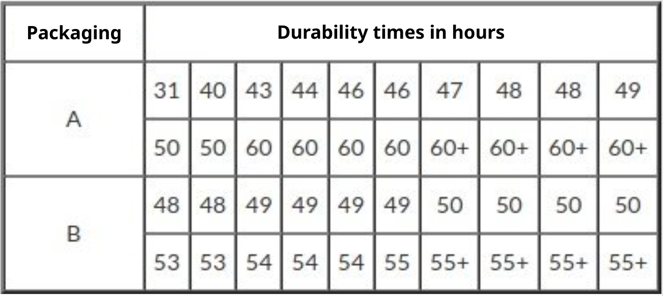
Is there a difference between the two packages in terms of product durability? Let’s compare the durability times using the Rank Test.
First, let’s organize the data in a new table, where we replace the + symbol with the indicator 0 (censure) and for the other values we put the indicator 1 (failure).
| Time | censorship | Groups |
|---|---|---|
| 31 | 1 | A |
| 40 | 1 | A |
| 43 | 1 | A |
| 44 | 1 | A |
| 46 | 1 | A |
| 46 | 1 | A |
| 47 | 1 | A |
| 48 | 1 | A |
| 48 | 1 | A |
| 49 | 1 | A |
| 50 | 1 | A |
| 50 | 1 | A |
| 60 | 1 | A |
| 60 | 1 | A |
| 60 | 1 | A |
| 60 | 1 | A |
| 60 | 0 | A |
| 60 | 0 | A |
| 60 | 0 | A |
| 60 | 0 | A |
| 48 | 1 | B |
| 48 | 1 | B |
| 49 | 1 | B |
| 49 | 1 | B |
| 49 | 1 | B |
| 49 | 1 | B |
| 50 | 1 | B |
| 50 | 1 | B |
| 50 | 1 | B |
| 50 | 1 | B |
| 53 | 1 | B |
| 53 | 1 | B |
| 54 | 1 | B |
| 54 | 1 | B |
| 54 | 1 | B |
| 55 | 1 | B |
| 55 | 0 | B |
| 55 | 0 | B |
| 55 | 0 | B |
| 55 | 0 | B |
We will upload the data to the system.
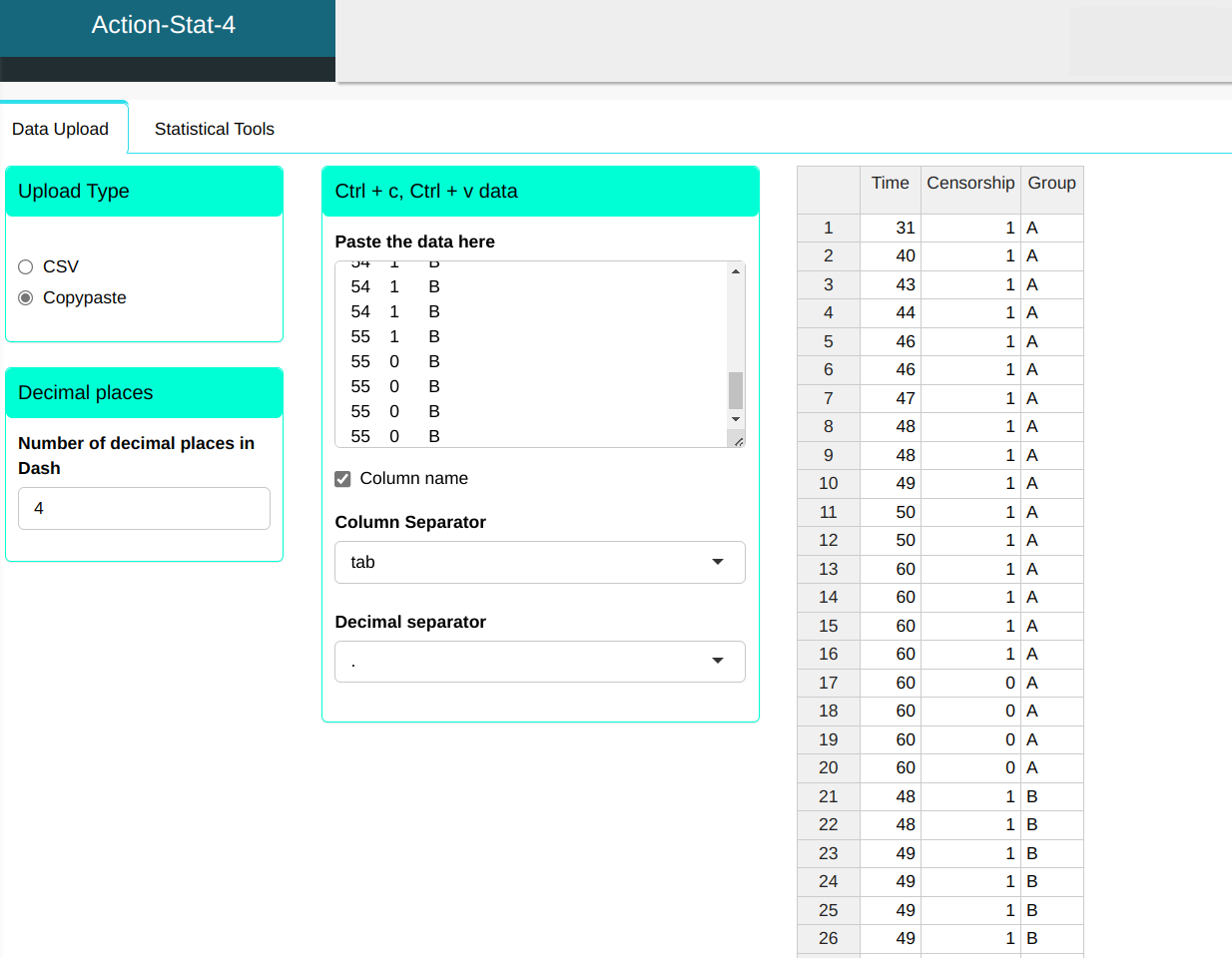
Configuring as shown in the figure below to perform the Rank test.
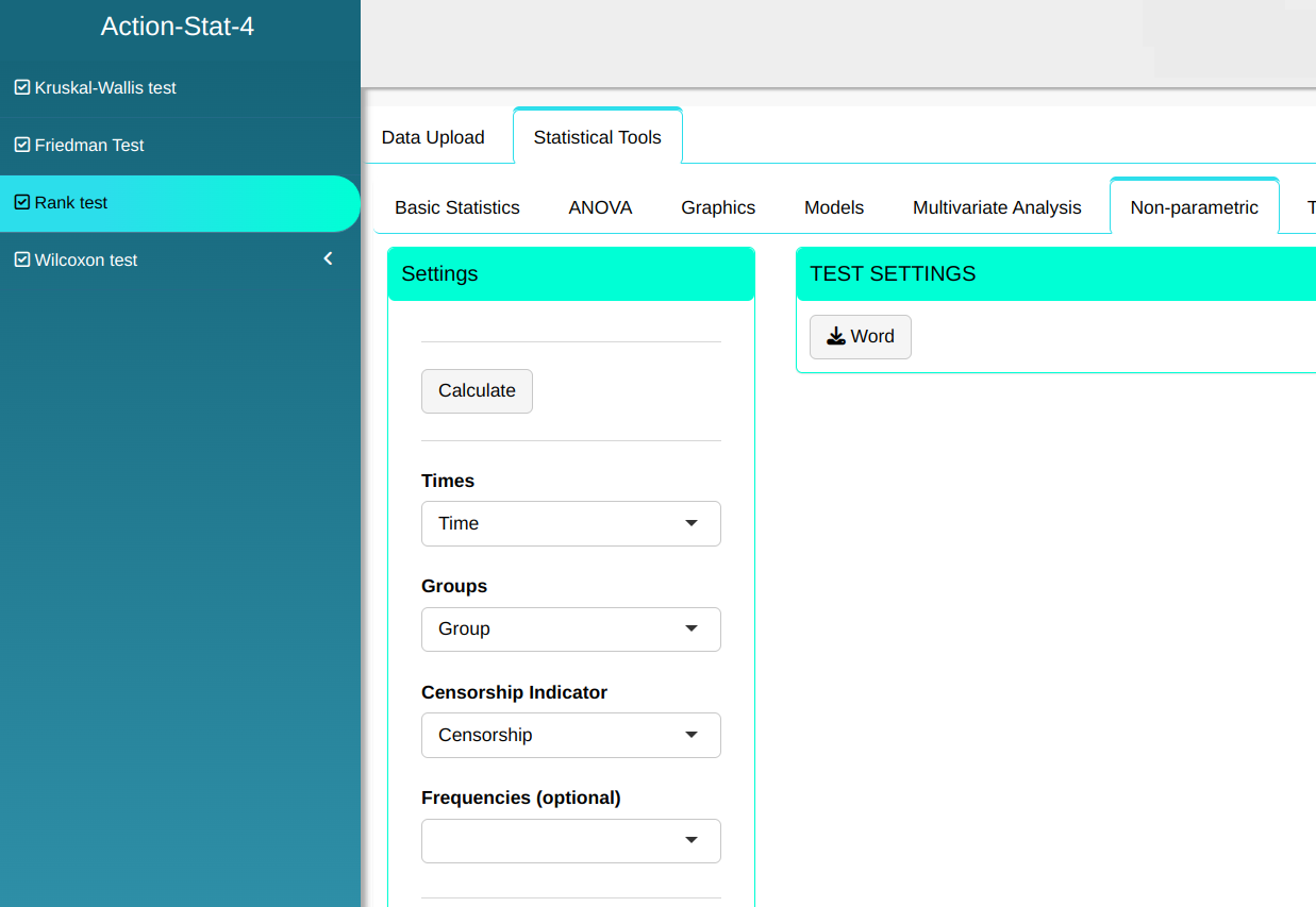
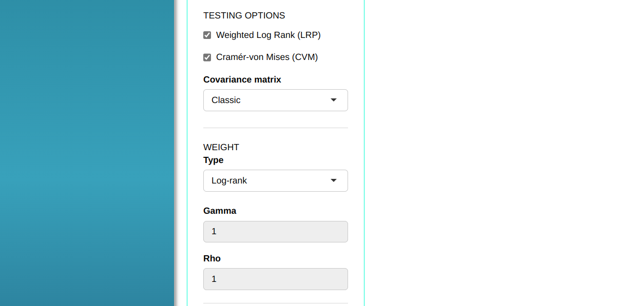
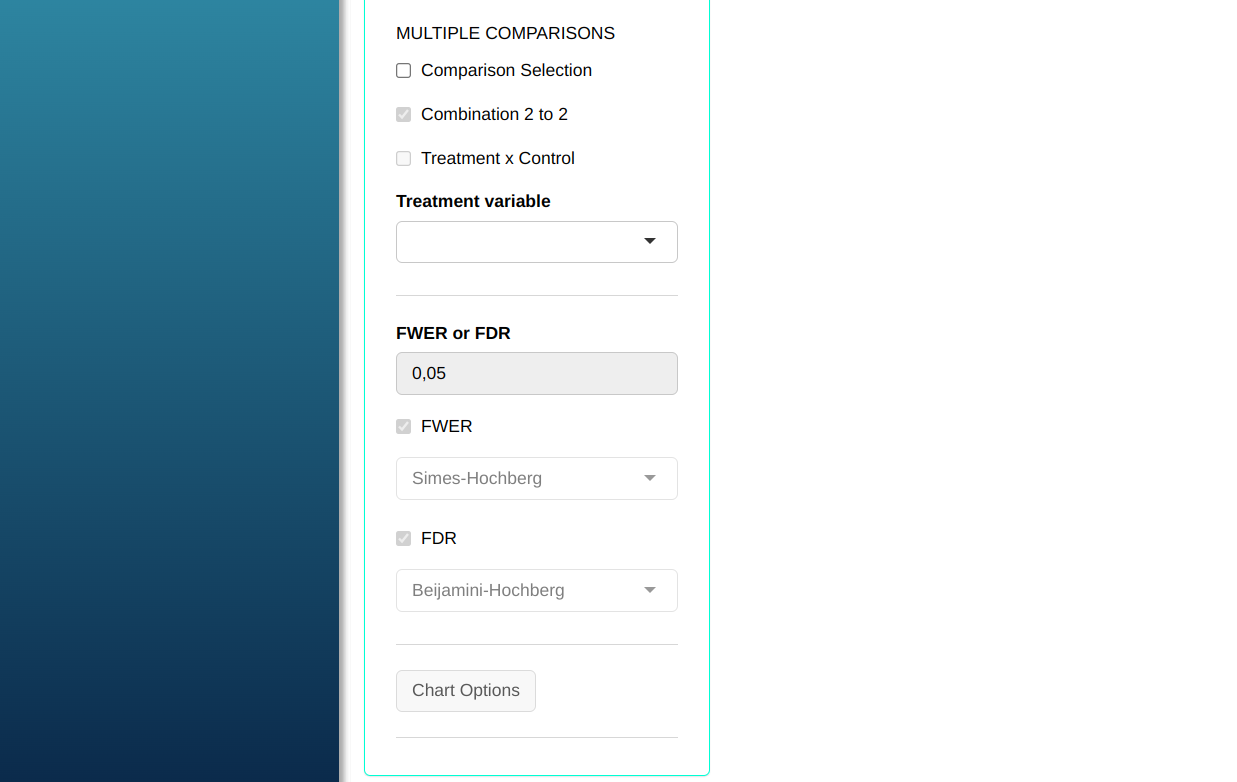
Then click Calculate to get the results. You can also generate the analyses and download them in Word format.

The results are
Comparison of groups
| Weight | Statistics | P-Value | |
|---|---|---|---|
| Cramér-von Mises (CVM) 1 | LogRank | 47.473 | 0.110 |
| Weightes Log-rank (LRP) 1 | LogRank | 0.006 | 0.936 |
Summary of comparison of groups
| Groups | Time | Number of events | Amount at risk | Standard Deviation | Survival Function | Lower Limit | Upper Limit | Hazard Function | Lower Limit.1 | Upper Limit.1 |
|---|---|---|---|---|---|---|---|---|---|---|
| A | 31.0000 | 1.0000 | 20.0000 | 0.0487 | 0.9500 | 0.8540 | 1.0000 | 0.0500 | 0.0452 | 0.0548 |
| A | 40.0000 | 1.0000 | 19.0000 | 0.0671 | 0.9000 | 0.7690 | 1.0000 | 0.1000 | 0.0869 | 0.1131 |
| A | 43.0000 | 1.0000 | 18.0000 | 0.0798 | 0.8500 | 0.6940 | 1.0000 | 0.1500 | 0.1265 | 0.1735 |
| A | 44.0000 | 1.0000 | 17.0000 | 0.0894 | 0.8000 | 0.6250 | 0.9750 | 0.2000 | 0.1649 | 0.2351 |
| A | 46.0000 | 2.0000 | 16.0000 | 0.1020 | 0.7000 | 0.4990 | 0.9010 | 0.3000 | 0.2397 | 0.3603 |
| A | 47.0000 | 1.0000 | 14.0000 | 0.1070 | 0.6500 | 0.4410 | 0.8590 | 0.3500 | 0.2768 | 0.4232 |
| A | 48.0000 | 2.0000 | 13.0000 | 0.1110 | 0.5500 | 0.3320 | 0.7680 | 0.4500 | 0.3519 | 0.5481 |
| A | 49.0000 | 1.0000 | 11.0000 | 0.1120 | 0.5000 | 0.2810 | 0.7190 | 0.5000 | 0.3904 | 0.6096 |
| A | 50.0000 | 2.0000 | 10.0000 | 0.1100 | 0.4000 | 0.1850 | 0.6150 | 0.6000 | 0.4712 | 0.7288 |
| A | 60.0000 | 4.0000 | 8.0000 | 0.0894 | 0.2000 | 0.0247 | 0.3750 | 0.8000 | 0.6598 | 0.9402 |
| B | 48.0000 | 2.0000 | 20.0000 | 0.0671 | 0.9000 | 0.7690 | 1.0000 | 0.1000 | 0.0869 | 0.1131 |
| B | 49.0000 | 4.0000 | 18.0000 | 0.1020 | 0.7000 | 0.4990 | 0.9010 | 0.3000 | 0.2397 | 0.3603 |
| B | 50.0000 | 4.0000 | 14.0000 | 0.1120 | 0.5000 | 0.2810 | 0.7190 | 0.5000 | 0.3904 | 0.6096 |
| B | 53.0000 | 2.0000 | 10.0000 | 0.1100 | 0.4000 | 0.1850 | 0.6150 | 0.6000 | 0.4712 | 0.7288 |
| B | 54.0000 | 3.0000 | 8.0000 | 0.0968 | 0.2500 | 0.0602 | 0.4400 | 0.7500 | 0.6077 | 0.8923 |
| B | 55.0000 | 1.0000 | 5.0000 | 0.0894 | 0.2000 | 0.0247 | 0.3750 | 0.8000 | 0.6598 | 0.9402 |
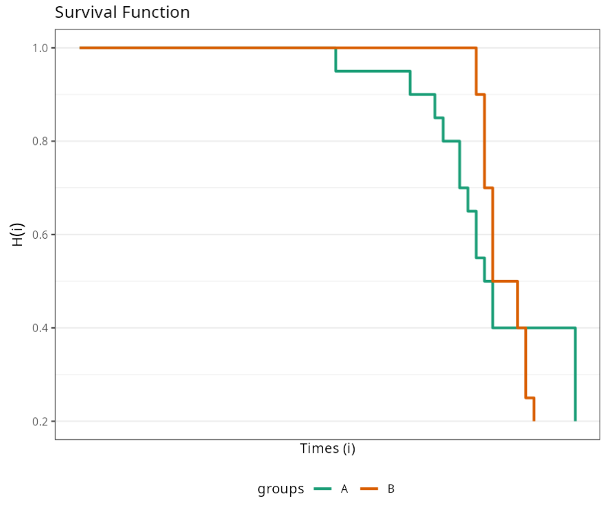
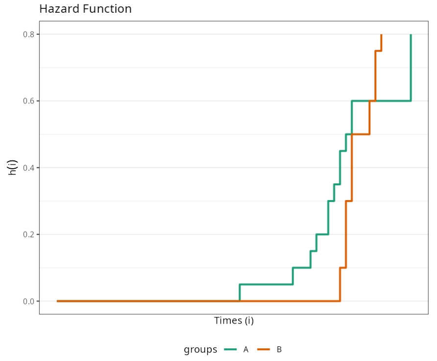
Knowing that the Rank Test is used to test the null hypothesis that there is no difference between groups (A and B), we conclude that, according to the p-value of 0.9362, we should not reject the null hypothesis. Thus, we say that there is no significant difference between the two packages with regard to the durability of the product.
Example 2:
A curd cheese producer carries out a shelf life test on his product. His product is sold at room temperature and without preservatives. The event of interest is the appearance of a fungus on the product. The data is shown below, with the time measured in hours. The + symbol indicates censorship.

Is there a difference between the two packages in terms of product durability? Let’s compare the durability times using the Rank Test.
To work with summarized data, we should set up the following table:
| Time | Censorship | Group | Frequency |
|---|---|---|---|
| 31 | 1 | A | 1 |
| 40 | 1 | A | 1 |
| 43 | 1 | A | 1 |
| 44 | 1 | A | 1 |
| 46 | 1 | A | 2 |
| 47 | 1 | A | 1 |
| 48 | 1 | A | 2 |
| 48 | 1 | B | 2 |
| 49 | 1 | A | 1 |
| 49 | 1 | B | 4 |
| 50 | 1 | A | 2 |
| 50 | 1 | B | 4 |
| 53 | 1 | B | 2 |
| 54 | 1 | B | 3 |
| 55 | 1 | B | 1 |
| 55 | 0 | B | 4 |
| 60 | 1 | A | 4 |
| 60 | 0 | A | 4 |
We will upload the data to the system.
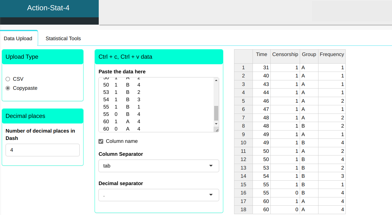
Configuring as shown in the figure below to perform the Rank test.
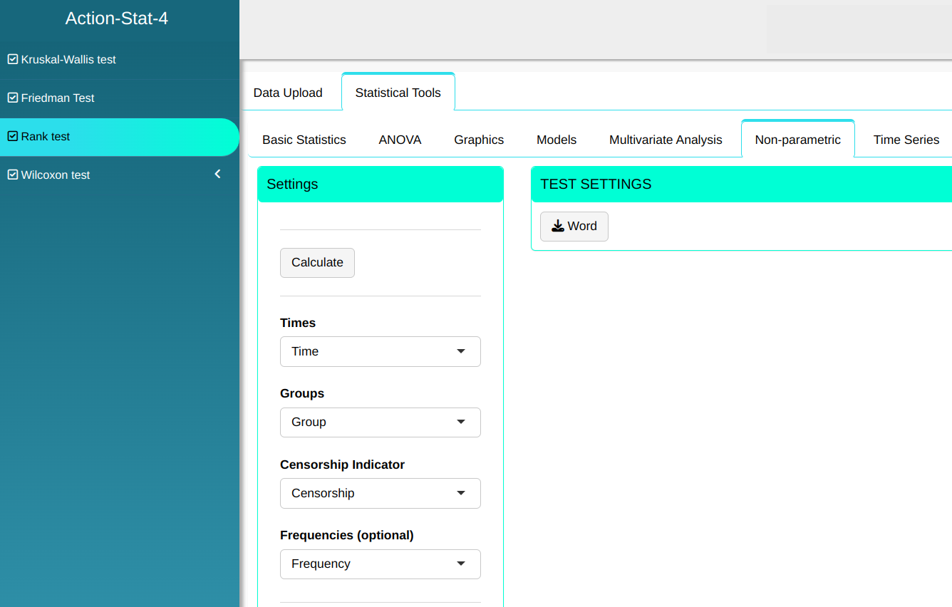

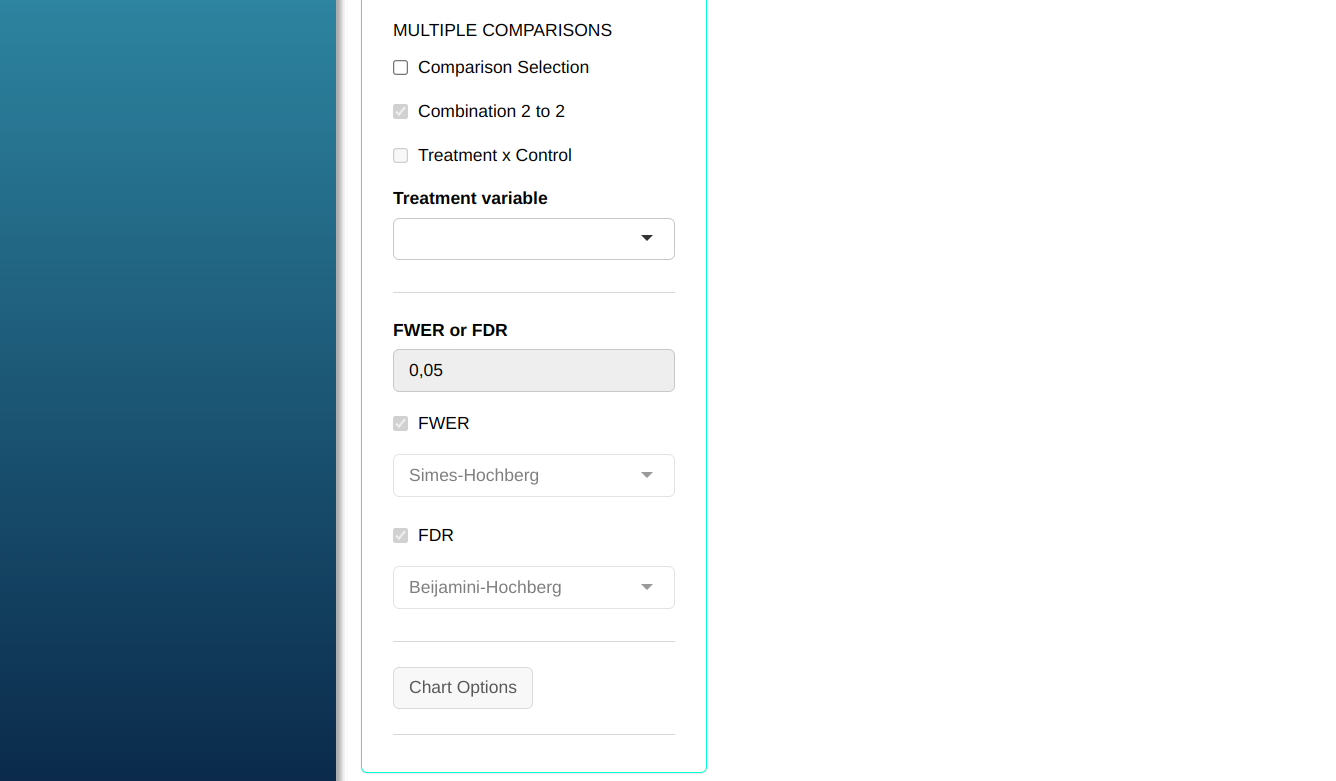
Then click Calculate to get the results. You can also generate the analyses and download them in Word format.

The results are:
Comparison of groups
| Weight | Statistics | P-Value | |
|---|---|---|---|
| Cramér-von Mises (CVM) 1 | LogRank | 47.473 | 0.110 |
| Weighted Log-rank (LRP) 1 | LogRank | 0.006 | 0.936 |
Summmary of comparison of groups
| Groups | Timeo | Number of events | Amount at risk | Standard Deviation | Survival Function | Lower Limit | Upper Limit | Hazard Function | Lower Limite.1 | Upper Limite.1 |
|---|---|---|---|---|---|---|---|---|---|---|
| A | 31 | 1 | 20 | 0.049 | 0.95 0.854 | 1 | 0.05 | 0.045 | 0.055 | |
| A | 40 | 1 | 19 | 0.067 | 0.9 | 0.769 | 1 | 0.1 | 0.087 | 0.113 |
| A | 43 | 1 | 18 | 0.08 | 0.85 | 0.694 | 1 | 0.15 | 0.127 | 0.173 |
| A | 44 | 1 | 17 | 0.089 | 0.8 | 0.625 | 0.975 | 0.2 | 0.165 | 0.235 |
| A | 46 | 2 | 16 | 0.102 | 0.7 | 0.499 | 0.901 | 0.3 | 0.24 | 0.36 |
| A | 47 | 1 | 14 | 0.107 | 0.65 0.441 | 0.859 | 0.35 | 0.277 | 0.423 | |
| A | 48 | 2 | 13 | 0.111 | 0.55 | 0.332 | 0.768 | 0.45 | 0.352 | 0.548 |
| A | 49 | 1 | 11 | 0.112 | 0.5 | 0.281 | 0.719 | 0.5 | 0.39 | 0.61 |
| A | 50 | 2 | 10 | 0.11 | 0.4 | 0.185 | 0.615 | 0.6 | 0.471 | 0.729 |
| A | 60 | 4 | 8 | 0.089 | 0.2 | 0.025 | 0.375 | 0.8 | 0.66 | 0.94 |
| B | 48 | 2 | 20 | 0.067 | 0.9 | 0.769 | 1 | 0.1 | 0.087 | 0.113 |
| B | 49 | 4 | 18 | 0.102 | 0.7 | 0.499 | 0.901 | 0.3 | 0.24 | 0.36 |
| B | 50 | 4 | 14 | 0.112 | 0.5 | 0.281 | 0.719 | 0.5 | 0.39 | 0.61 |
| B | 53 | 2 | 10 | 0.11 | 0.4 | 0.185 | 0.615 | 0.6 | 0.471 | 0.729 |
| B | 54 | 3 | 8 | 0.097 | 0.25 | 0.06 | 0.44 | 0.75 | 0.608 | 0.892 |
| B | 55 | 1 | 5 | 0.089 | 0.2 | 0.025 | 0.375 | 0.8 | 0.66 | 0.94 |
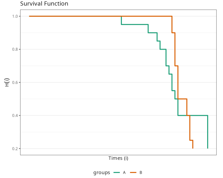
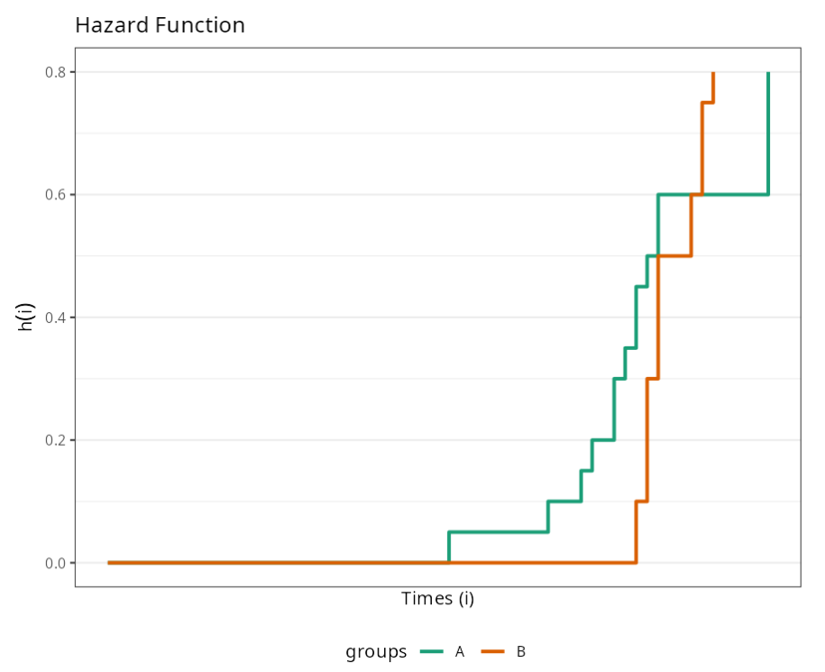
Knowing that the Rank test is used to test the null hypothesis that there is no difference between groups (A and B), we conclude that, according to the p-value of 0.5399, we should not reject the null hypothesis. Thus, we say that there is no significant difference between the two packages with regard to the durability of the product.