4. Wilcoxon Test
Using the Wilcoxon test, we tested the pseudo medians, for the sample single, independent and paired samples.
Example 1:
Assuming that the sample numbers are symmetrically distributed in around the median, we will use the Wilcoxon test to test the hypothesis $H_0: θ_0$ = 220 where the median is equal to 220, at the significance level of 5%.
| Data |
|---|
| 126 |
| 142 |
| 156 |
| 228 |
| 245 |
| 246 |
| 370 |
| 419 |
| 433 |
| 454 |
| 478 |
| 503 |
We will upload the data to the system.
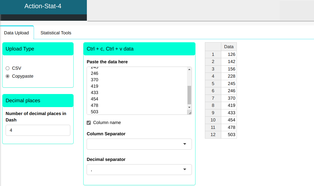
The Wilcoxon test will be conducted using the settings shown in the figure below.


Then click Calculate to get the results. You can also generate the analyses and download them in Word format.

The results are:
Statistics Table (Wilcoxon)
| Values | |
|---|---|
| Statistics | 63 |
| P-value | 0.064 |
| Null Hypothesis | 220 |
| Lower Limit | 200.5 |
| (Pseudo) Median | 315.75 |
| Upper Limit | 433 |
| Confidence Level | 0.95 |
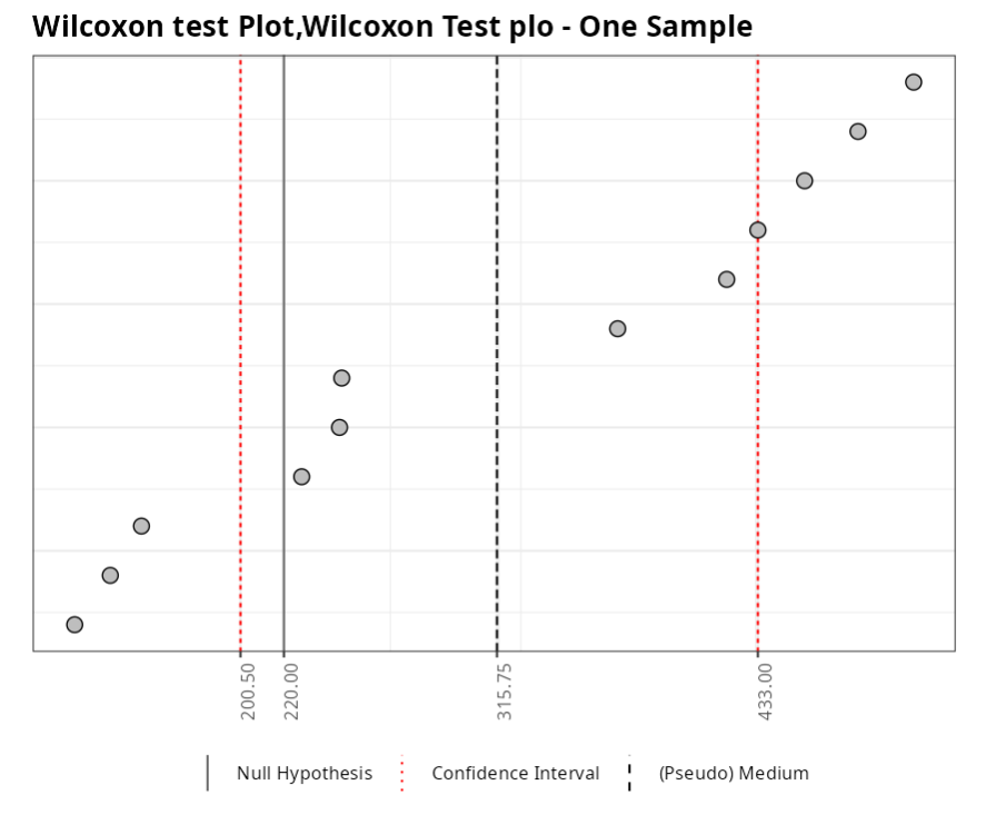
The test statistic is V = 63, As the p-value is equal to 0.0639 = 6.39% > 5% we do not reject the null hypothesis that $θ_0$ = 220 at the level of 5% significance.
Example 2:
Two samples provided the following values for a certain variable,
| Samples | Data |
|---|---|
| Sample 1 | 29 |
| Sample 1 | 39 |
| Sample 1 | 60 |
| Sample 1 | 78 |
| Sample 1 | 82 |
| Sample 1 | 112 |
| Sample 1 | 125 |
| Sample 1 | 170 |
| Sample 1 | 192 |
| Sample 1 | 224 |
| Sample 1 | 263 |
| Sample 1 | 275 |
| Sample 1 | 276 |
| Sample 1 | 286 |
| Sample 1 | 369 |
| Sample 1 | 756 |
| Sample 2 | 126 |
| Sample 2 | 142 |
| Sample 2 | 156 |
| Sample 2 | 228 |
| Sample 2 | 245 |
| Sample 2 | 246 |
| Sample 2 | 370 |
| Sample 2 | 419 |
| Sample 2 | 433 |
| Sample 2 | 454 |
| Sample 2 | 478 |
| Sample 2 | 503 |
We will upload the data to the system,
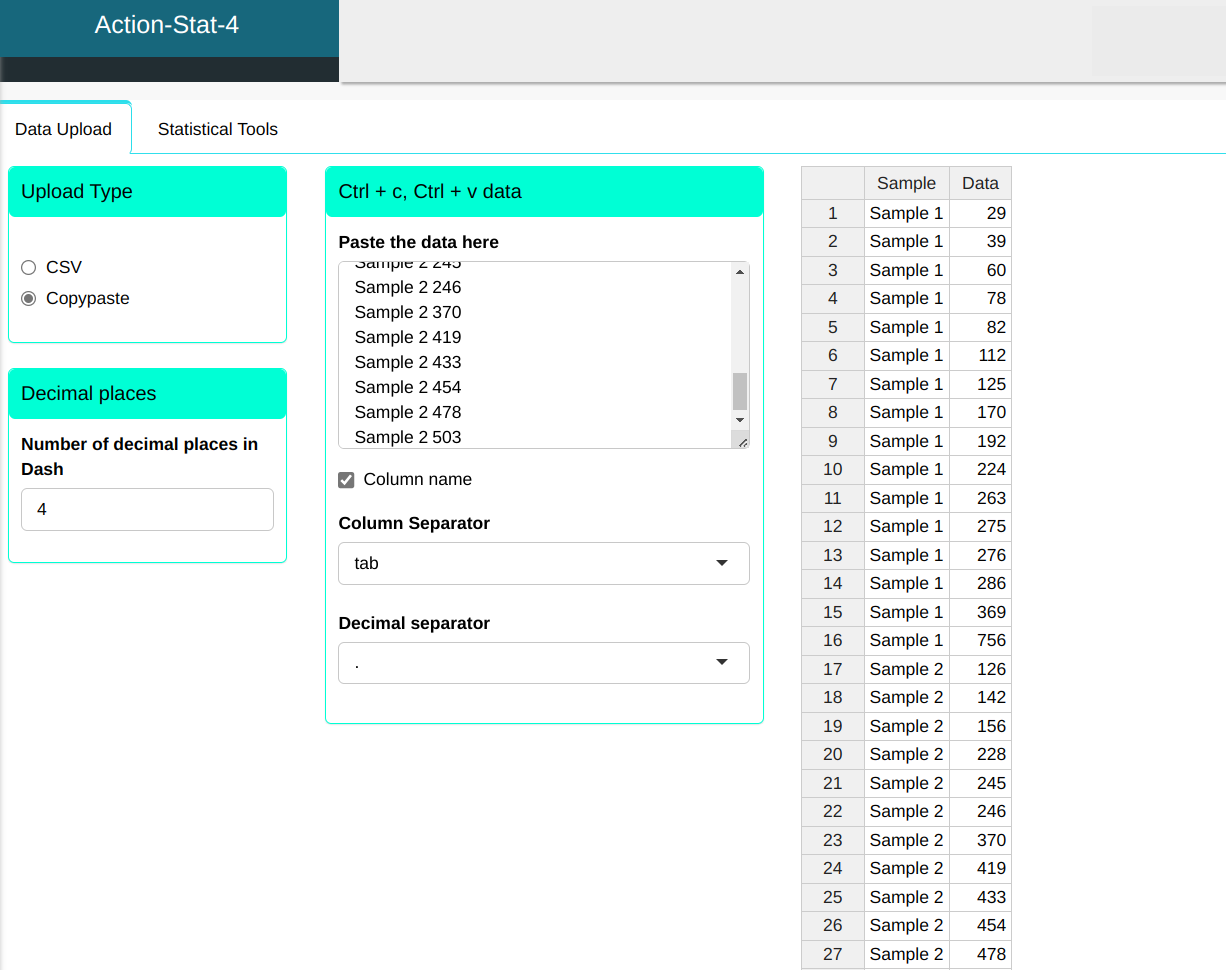
The Wilcoxon test will be conducted using the settings shown in the figure below.


Then click Calculate to get the results. You can also generate the analyses and download them in Word format.
The results are:
Statistics Table (Wilcoxon)
| Values | |
|---|---|
| Statistics | 141 |
| P-value | 0.0373 |
| Null Hypothesis | 0 |
| Lower Limit | 4 |
| (Pseudo) Median | 133.5 |
| Upper Limit | 240 |
| Confidence Level | 0.95 |
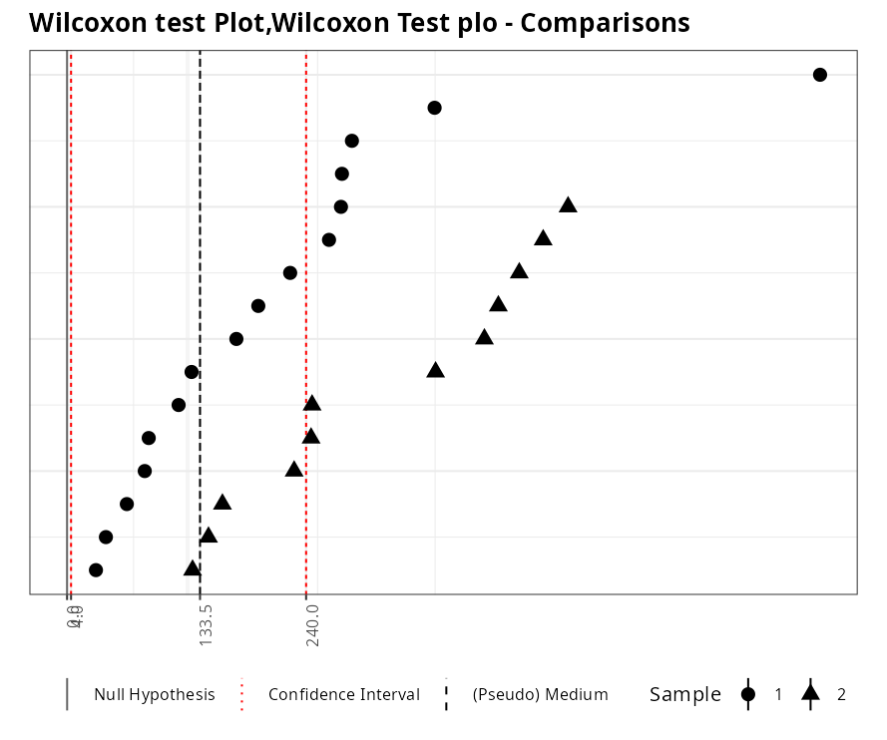
The test statistic is W = 141, Since the p-value is equal to 0.0373 = 3.73% < 5%, we reject the null hypothesis, Thus, we have evidence that the samples come from populations that have different medians.
Example 3:
Let us consider two dependent samples whose data are in the table. Is there evidence of a difference between the two samples?
| Sample 1 | Sample 2 |
|---|---|
| 564 | 557 |
| 521 | 505 |
| 495 | 465 |
| 564 | 562 |
| 560 | 545 |
| 481 | 448 |
| 545 | 531 |
| 478 | 458 |
| 580 | 562 |
| 484 | 485 |
| 539 | 520 |
| 467 | 445 |
We will upload the data to the system.
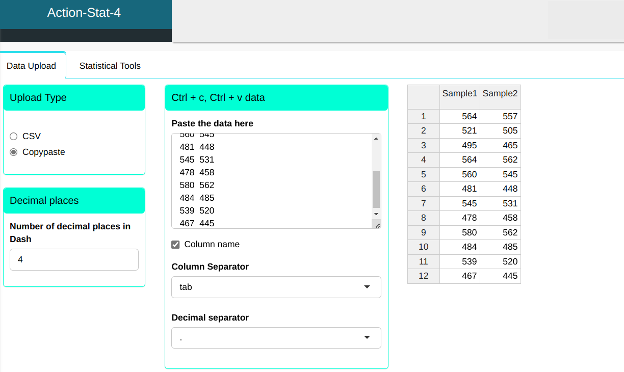
The Wilcoxon test will be conducted using the settings shown in the figure below.


Then click Calculate to get the results. You can also generate the analyses and download them in Word format.
The results are:
Test Statistics Table (Wilcoxon)
| Values | |
|---|---|
| Statistics | 77 |
| P-value | 0.001 |
| Null Hypothesis | 0 |
| Lower Limit | 9 |
| (Pseudo) Median | 16.5 |
| Upper Limit | 23.5 |
| Confidence Level | 0.95 |
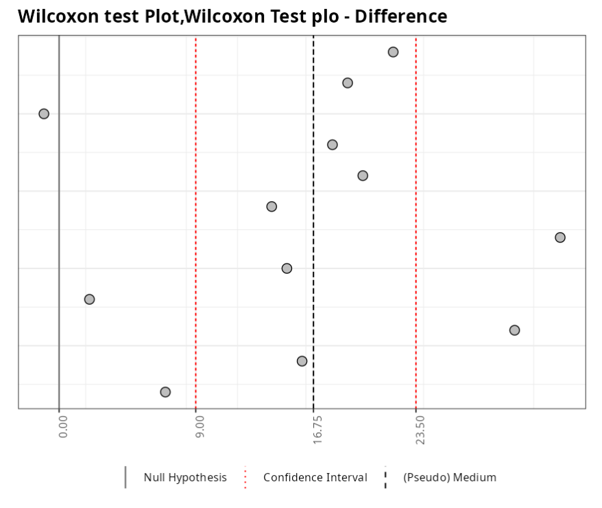
The test statistic is W = 77. As the P-value = 0.000976563 < 5%. So, at the 5% significance level, there is evidence of a difference between the two samples.