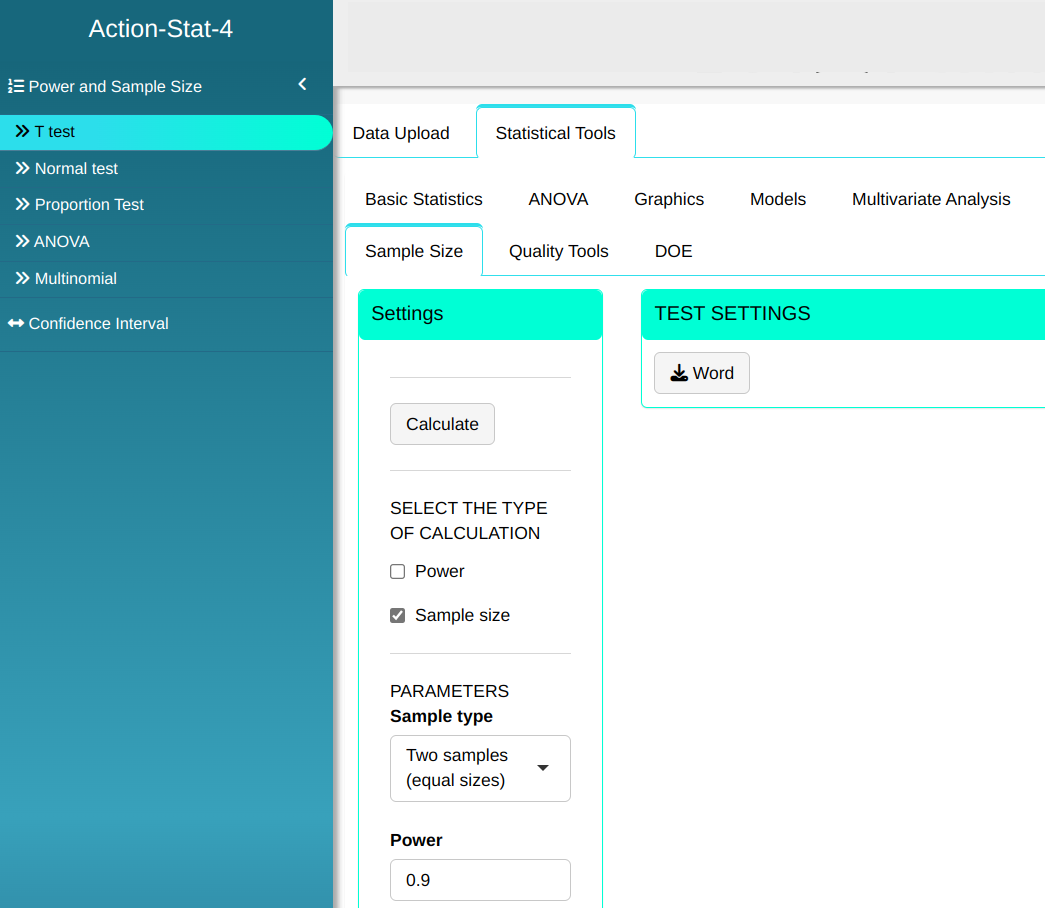
1. Teste T
Here the T-Test is used to calculate the power of the hypothesis test or the sample size.
Example 1:
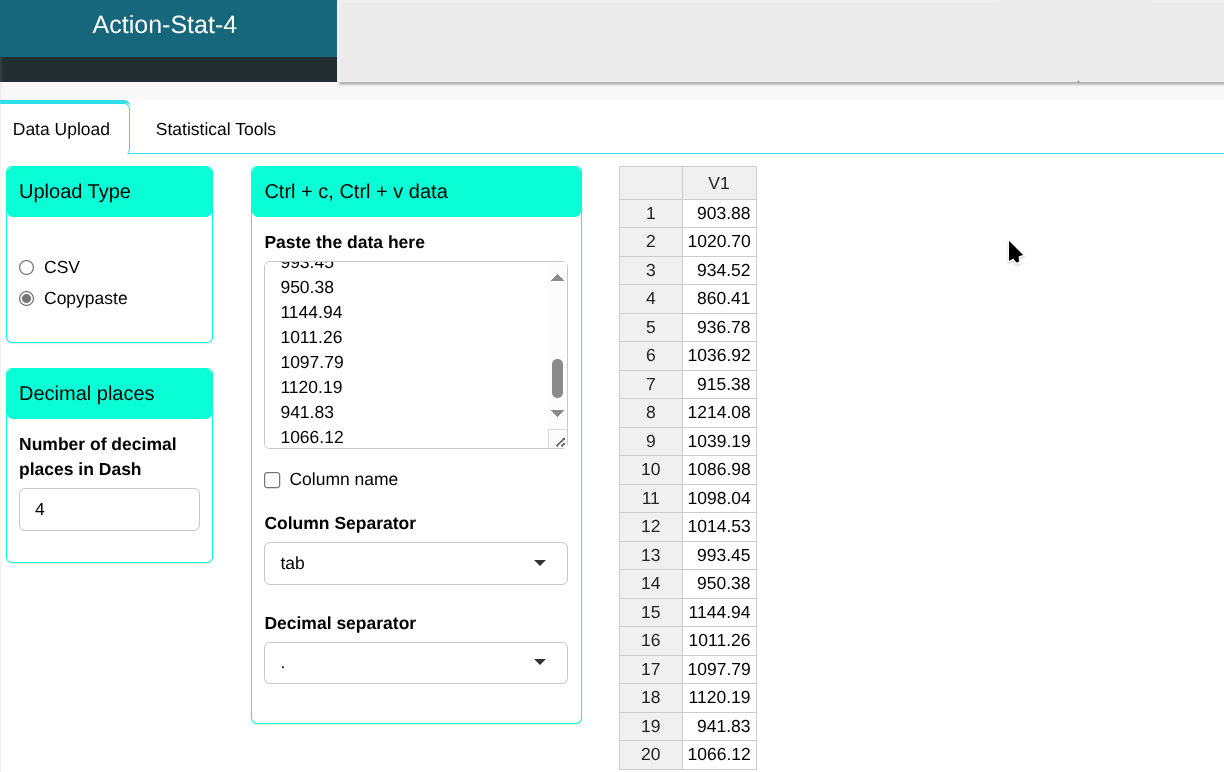
A production engineer intends to test, based on the data in the following table and for a significance level $\alpha$ = 0.05, whether the average height of a rod is close to the nominal value of 1055mm. To this end, a sample of 20 rods was analyzed, whose measurements are found in the table.
| 903.88 |
| 1020.7 |
| 934.52 |
| 860.41 |
| 936.78 |
| 1036.92 |
| 915.38 |
| 1214.08 |
| 1039.19 |
| 1086.98 |
| 1098.04 |
| 1014.53 |
| 993.45 |
| 950.38 |
| 1144.94 |
| 1011.26 |
| 1097.79 |
| 1120.19 |
| 941.83 |
| 1066.12 |
Neste caso, estabelecemos as hipóteses
- $H_0$: $\mu =$ 1055
- $H_1$: $\mu \neq $ 1055
Using the Descriptive Summary tool in Action Basic Statistics menu, we find that the sample mean is $\overline{X}$=1019.3685 and the sample standard deviation is s = 91.36863255.
We will then calculate the power of the T-test considering the following values
| $\quad\mathbf{\sigma}$ | $\mathbf{n}$ | nivel de significancia |
| 91.37 | 20 | $\qquad \quad$ 0.05 |
To calculate the Power of a hypothesis test, we calculate the probability of rejecting the null hypothesis when it is really false, i.e. the alternative hypothesis is true. Thus, we assume a value x for the alternative hypothesis and the power of the test is the probability that the test has of detecting the difference d between the value x of the alternative hypothesis and the value of the null hypothesis.
We will upload the data to the system.
Configuring as shown in the figure below to perform the test.
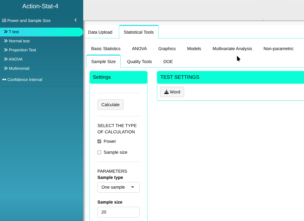

Then click Calculate we obtain the results. You can also generate the test and download them in Word format.

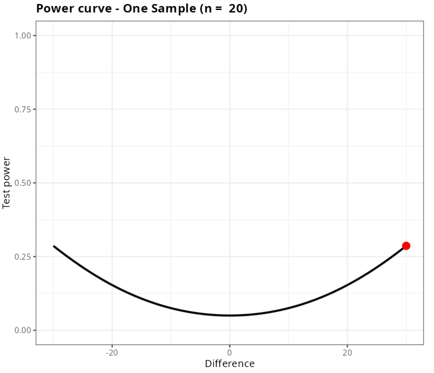
The results are:
T-Test - One sample
| V1 | |
|---|---|
| Power | 0.2863009 |
| Sample size | 20 |
| Difference | 30 |
| Significance Level | 0.05 |
| Standard deviation | 91.37 |
| Alternative Hyphotesis | Different |
Example 2:
Using the same data in the previous example, suppose now that we want to calculate the sample size needed for the T-test to detect a difference of 30mm with at least 90% power.
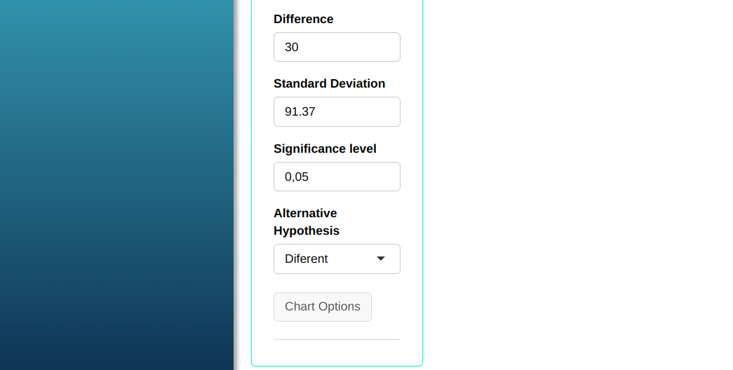
Configuring as shown in the figure below to perform the test.
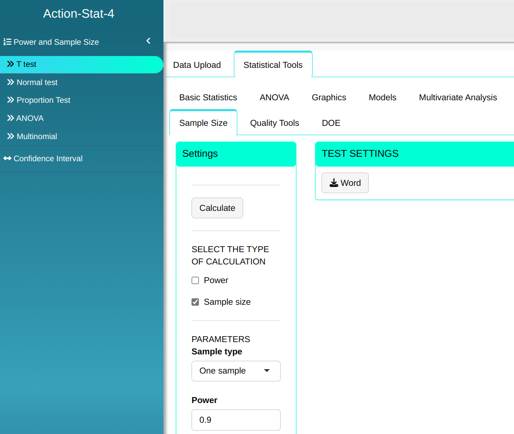
Then click Calculate we obtain the results. You can also generate the test and download them in Word format.
The results are:
T-Test - One sample
| V1 | |
|---|---|
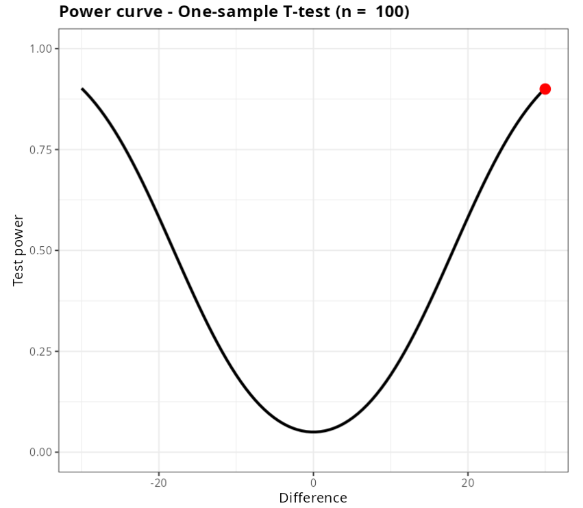
| Power | 0.9 |
| Sample size | 100 |
| Difference | 30 |
| Singnificance Level | 0.05 |
| Standard Deviation | 91.37 |
| Alternative Hyphotesis | Different |
Example 3:
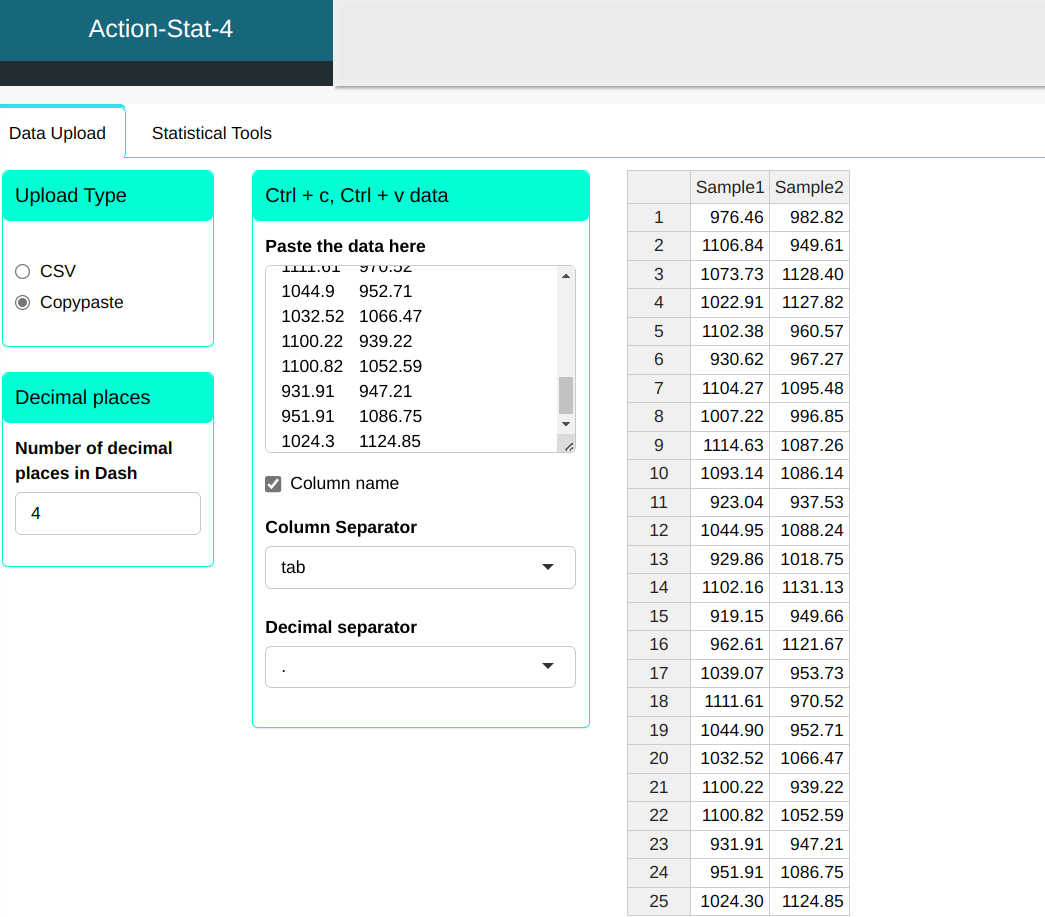
Considering the data below, compare the sample averages.
| Sample 1 | Sample 2 |
|---|---|
| 976.46 | 982.82 |
| 1106.84 | 949.61 |
| 107.73 | 1128.40 |
| 1022.91 | 1127.82 |
| 1102.38 | 960.57 |
| 930.62 | 967.27 |
| 1104.27 | 1095.48 |
| 1007.22 | 996.85 |
| 1114.63 | 1087.26 |
| 1093.14 | 1086.14 |
| 923.04 | 937.53 |
| 1044.95 | 1088.24 |
| 929.86 | 1018.75 |
| 1102.16 | 1131.13 |
| 919.15 | 949.66 |
| 962.61 | 1121.67 |
| 1039.07 | 953.73 |
| 1111.61 | 970.52 |
| 1044.90 | 952.71 |
| 1032.52 | 1066.47 |
| 1100.22 | 939.22 |
| 1100.82 | 1052.59 |
| 931.91 | 947.21 |
| 951.91 | 1086.75 |
| 1024.30 | 1124.85 |
Establishing hypotheses:
- $ H_0$: $\mu_1 -\mu_2$ = 0
- $ H_1$: $\mu_1$ -$\mu_2$ $\neq$ 0
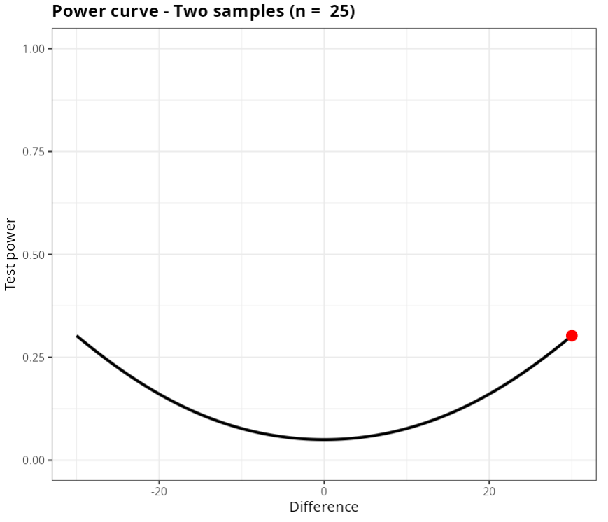
Let us calculate the power of the T-test, with two samples of the same size, to detect a difference $\mu_1$ -$\mu_2$ = 30. First, we need to calculate the standard deviation. Using Action Descriptive Summary tool, we obtain the following values $s_1$ = 70.54 e $s_2$ = 73.63
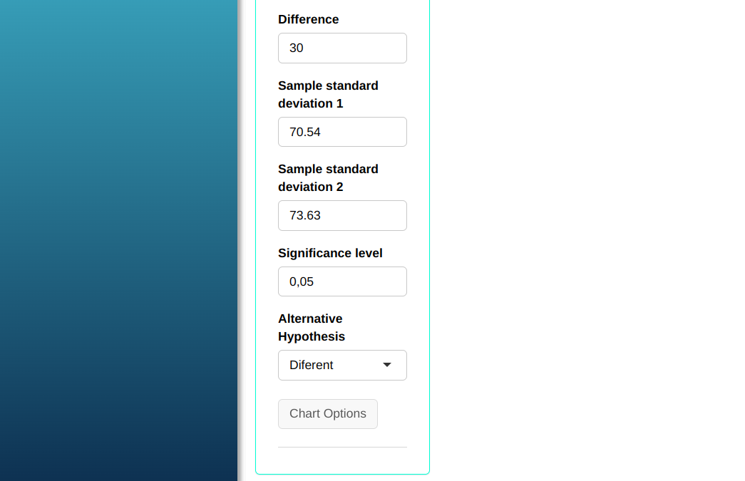
| $\mathbf{n_1 = n_2}$ | $\mathbf{\alpha}$ | Diferença $\mathbf{(\mu_1 - \mu_2)}$ | Desvio-Padrão 1 | Desvio-Padrão 2 |
| $\quad$ 25 | 0.05 | $\qquad$ 30 | $\quad \quad$ 70.54 | $\qquad$ 73.63 |
We will upload the data to the system.
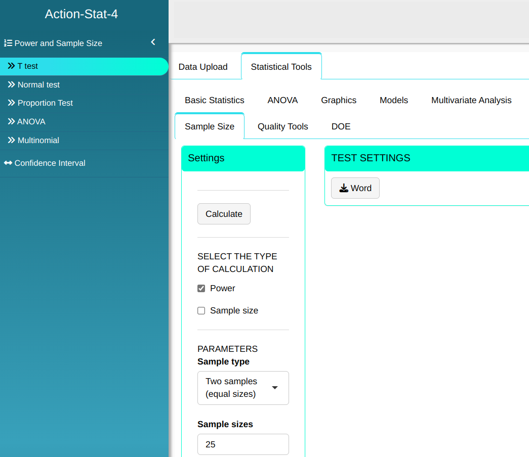
Configuring as shown in the figure below to perform the test.
Then click Calculate we obtain the results. You can also generate the test and download them in Word format.
The results are:
Two-Sample T-test (Equal size)
| V1 | |
|---|---|
| Power | 0.302466 |
| Sample size | 25 |
| Difference | 30 |
| Standard Deviation 1 | 70.54 |
| Standard Deviation 2 | 73.63 |
| Significance Level | 0.05 |
| Alternative Hyphotesis | Different |
Example 4:
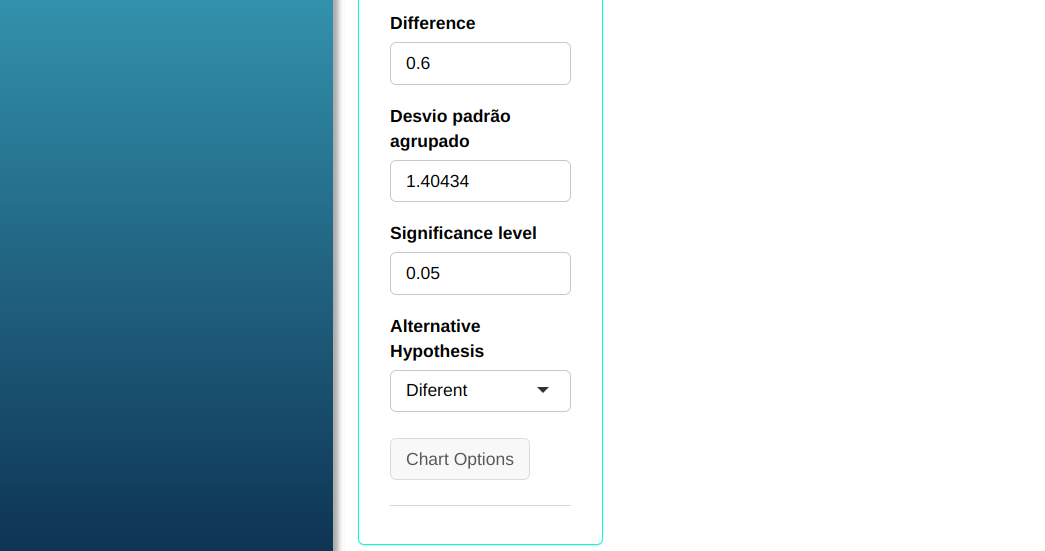
Now suppose, with the same set of data, we want to calculate the sample size needed to detect a difference $\mu_1 - \mu_2 = $ 0.6 with a power of minimum 0.9 and a standard deviation of 1.40434.
| Poder | $\mathbf{\alpha}$ | Diferença $\mathbf{(\mu_1 - \mu_2)}$ | Desvio-Padrão sp | |
| $\quad$ 0,9 | 0,05 | $\qquad \quad$ 0,6 | $\quad \quad$ 1,40434 |
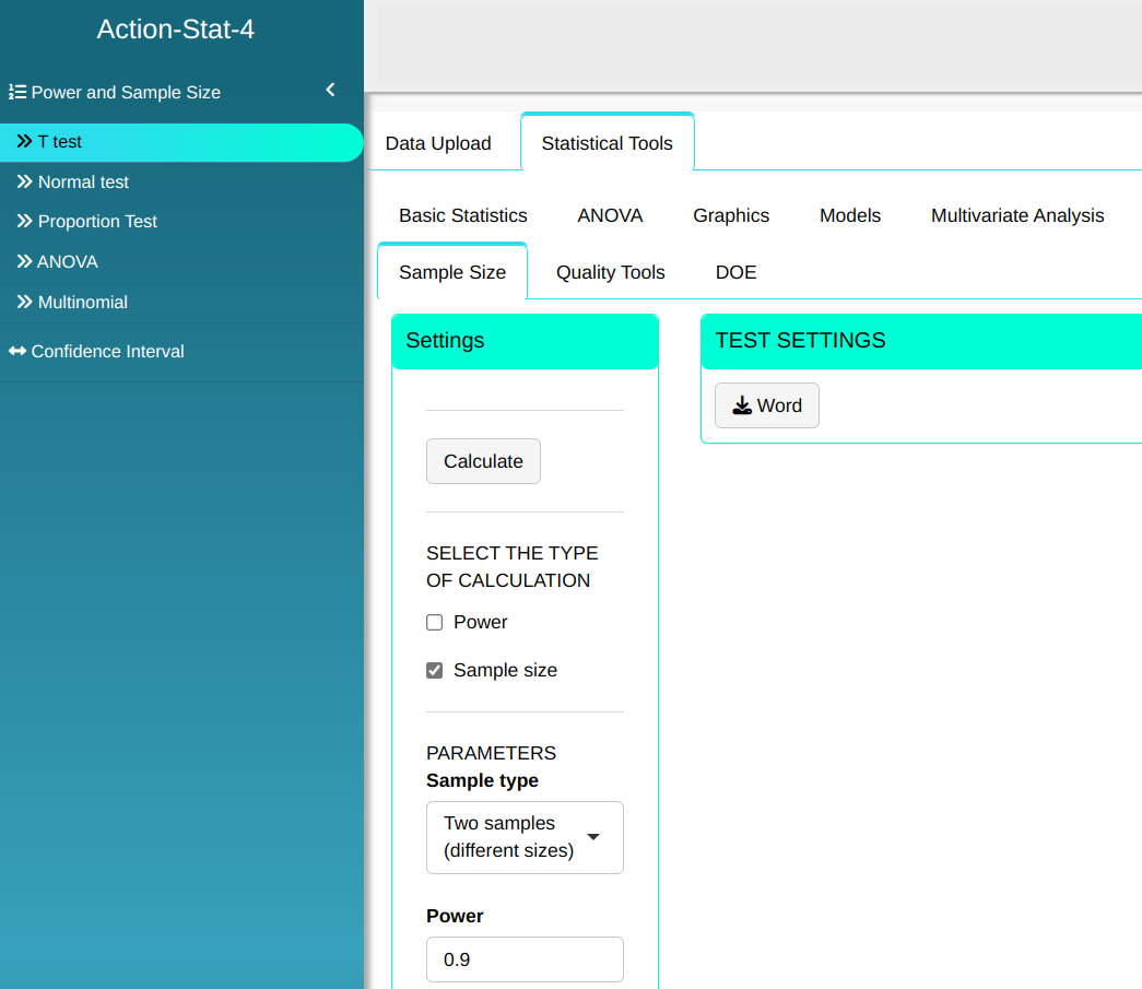
Configuring as shown in the figure below to perform the test.
Then click Calculate we obtain the results. You can also generate the test and download them in Word format.
The results are:
Two-Sample T-test (Equal size)
| V1 | |
|---|---|
| Power | 0.9 |
| Sample size | 117 |
| Difference | 0.6 |
| Standard Deviation | 1.40434 |
| Significance Level | 0.05 |
| Alternative Hyphotesis | Different |
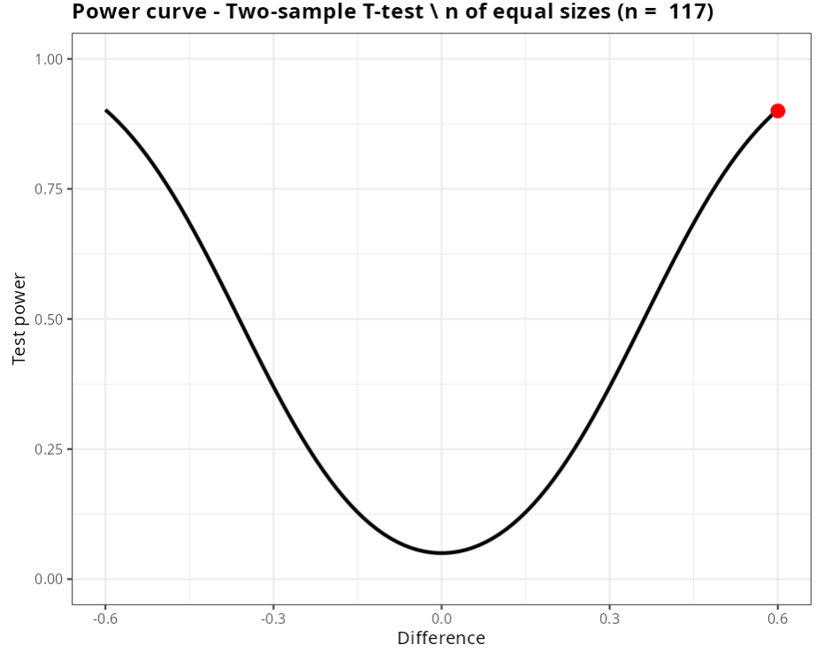
We conclude that, to detect a difference of 0.6 with a power of minimum 0.9, the two samples must have 117 elements.
Example 5:
Compare the averages of the samples whose measurements are presented in the following tables.
| Data | Sample |
|---|---|
| 18.8 | Sample 1 |
| 20.504 | Sample 1 |
| 18.621 | Sample 1 |
| 19.919 | Sample 1 |
| 21.117 | Sample 1 |
| 17.591 | Sample 1 |
| 18.756 | Sample 1 |
| 18.977 | Sample 1 |
| 20.308 | Sample 1 |
| 18.899 | Sample 1 |
| 20.835 | Sample 1 |
| 17.527 | Sample 1 |
| 17.078 | Sample 1 |
| 17.62 | Sample 1 |
| 21.426 | Sample 1 |
| 19.169 | Sample 1 |
| 19.29 | Sample 1 |
| 22.059 | Sample 1 |
| 18.585 | Sample 1 |
| 17.89 | Sample 1 |
| 18.755 | Sample 1 |
| 19.203 | Sample 1 |
| 18.419 | Sample 1 |
| 20.764 | Sample 1 |
| 21.055 | Sample 1 |
| 22.284 | Sample 2 |
| 21.901 | Sample 2 |
| 25.302 | Sample 2 |
| 22.447 | Sample 2 |
| 22.771 | Sample 2 |
| 22.057 | Sample 2 |
| 22.881 | Sample 2 |
| 17.968 | Sample 2 |
| 23.382 | Sample 2 |
| 21.043 | Sample 2 |
| 22.629 | Sample 2 |
| 22.86 | Sample 2 |
| 24.515 | Sample 2 |
| 22.426 | Sample 2 |
| 21.203 | Sample 2 |
| 24.62 | Sample 2 |
| 22.058 | Sample 2 |
| 23.15 | Sample 2 |
| 22.787 | Sample 2 |
| 24.009 | Sample 2 |
| 21.491 | Sample 2 |
| 22.699 | Sample 2 |
| 24.662 | Sample 2 |
| 21.983 | Sample 2 |
| 21.917 | Sample 2 |
| 21.198 | Sample 2 |
| 22.909 | Sample 2 |
| 23.327 | Sample 2 |
| 24.534 | Sample 2 |
| 21.152 | Sample 2 |
Establish hypotheses:
- $H_0$: $\mu_1 - \mu_2 = $ 0
- $H_1$: $\mu_1 - \mu_2 \neq $ 0
First, we need to calculate the standard deviation. Using Action Descriptive Summary tool, we get the values $s_1 =$ 1.36228 e $s_2 =$ 1.43822
Let us calculate the power of the two-sample T-test to detect a difference μ1 - μ2 = 1,5.
| $\mathbf{n_1}$ | $\mathbf{n_2}$ | $\mathbf{\alpha}$ | Diferença $\mathbf{(\mu_1 - \mu_2)}$ | Desvio-Padrão 1 | Desvio-Padrão 2 |
| 25 | 30 | 0.05 | $\qquad \quad$ 1.5 | $\qquad$ 1.36228 | $\quad$ 1.43822 |
We will upload the data to the system.
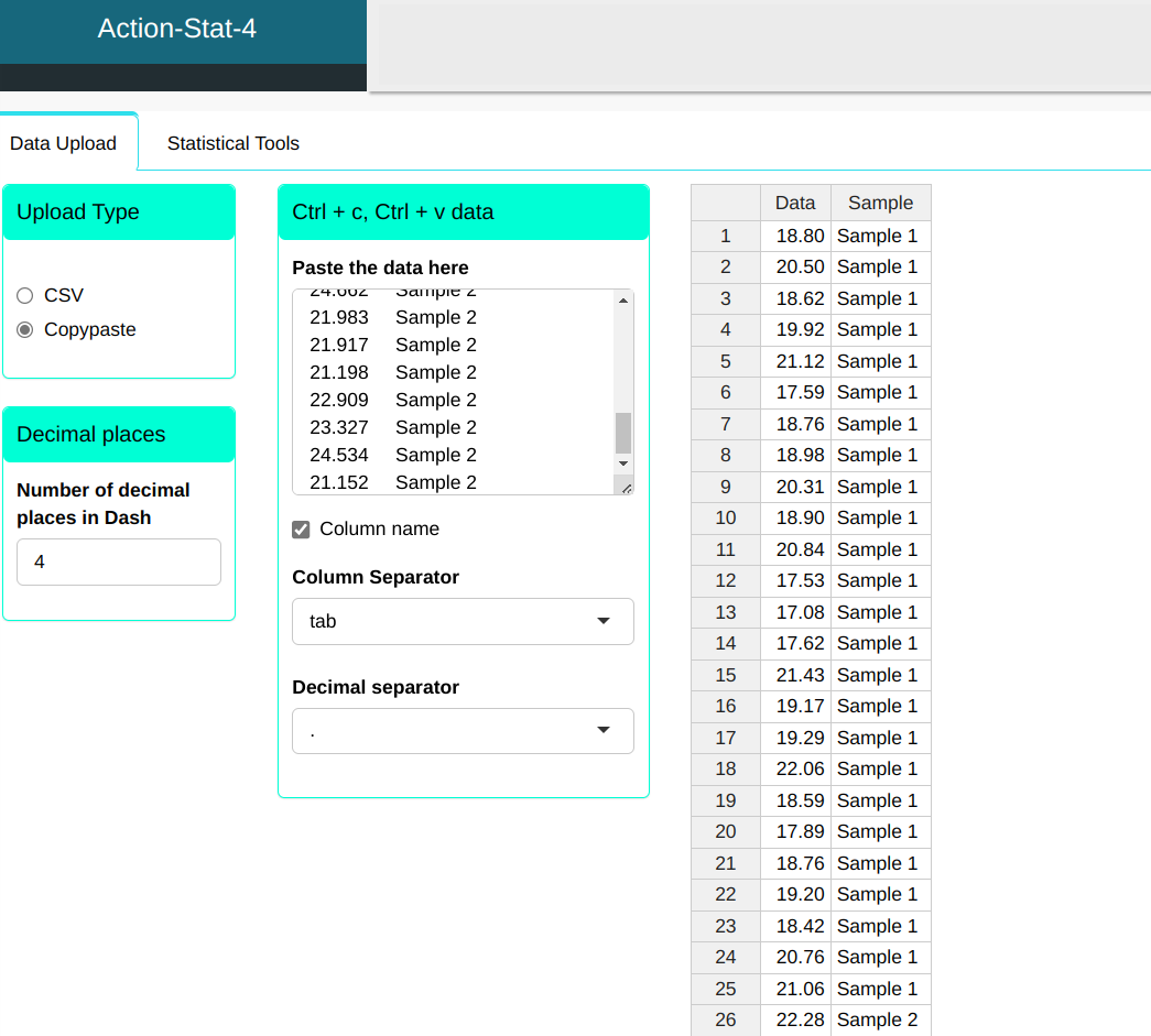
Configuring as shown in the figure below to perform the test.
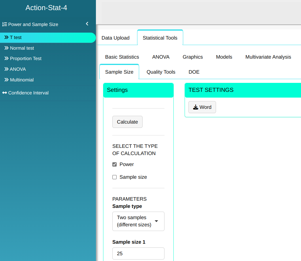
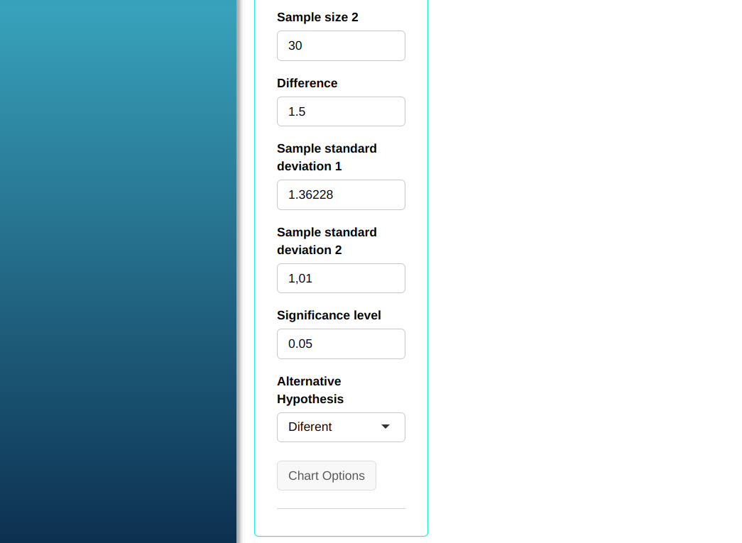
Then click Calculate we obtain the results. You can also generate the test and download them in Word format.
The results are:
Two-Sample T-test - different Size
| V1 | |
|---|---|
| Poder | 0.9720551 |
| Sample size 1 | 25 |
| Sample size 2 | 30 |
| Difference | 1.5 |
| Standard Deviation 1 | 1.36228 |
| Standard Deviation 2 | 1.43822 |
| Nível de significância | 0.05 |
| Alternative Hyphotesis | Different |
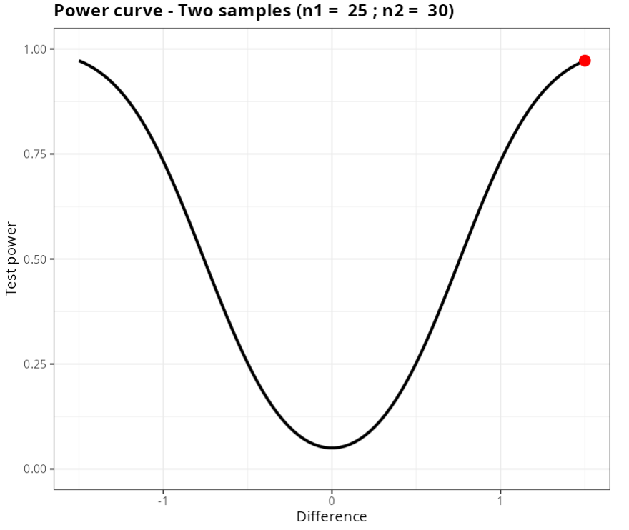
In other words, to detect a difference of d = 1.5 between the means, this test has a power of 97.20%
Example 6:
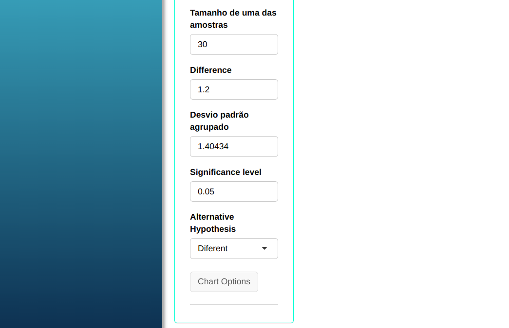
Using the previous example, suppose that with a sample size of 30, pooled standard deviation 1.40434, we want to calculate the size of the other sample needed for the T-test to find a difference of 1.2, with a power of at minimum 90%.
| Poder | $\mathbf{\alpha}$ | Difference $\mathbf{(\mu_1 - \mu_2)}$ | Standard Deviation | |
| $\quad$ 0.9 | 0.05 | $\qquad \quad$ 1.2 | $\quad \quad$ 1.40434 |
Configuring as shown in the figure below to perform the test.
Then click Calculate we obtain the results. You can also generate the test and download them in Word format.
The results are:
Two-Sample T-test (different Size)
| V1 | |
|---|---|
| Power | 0.9 |
| Sample size 1 | 30 |
| Sample size 2 | 30 |
| Difference | 1.2 |
| Standard Deviation | 1.40434 |
| Significance Level | 0.05 |
| Alternative Hyphotesis | Different |
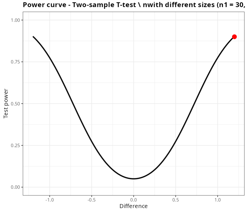
Concluímos então que, com uma das amostras com 30 elementos, para detectar uma diferença de 1,2 com um poder de, no mínimo, 90%, é necessário que a outra amostra também tenha aproximadamente 30 elementos.
Example 7:
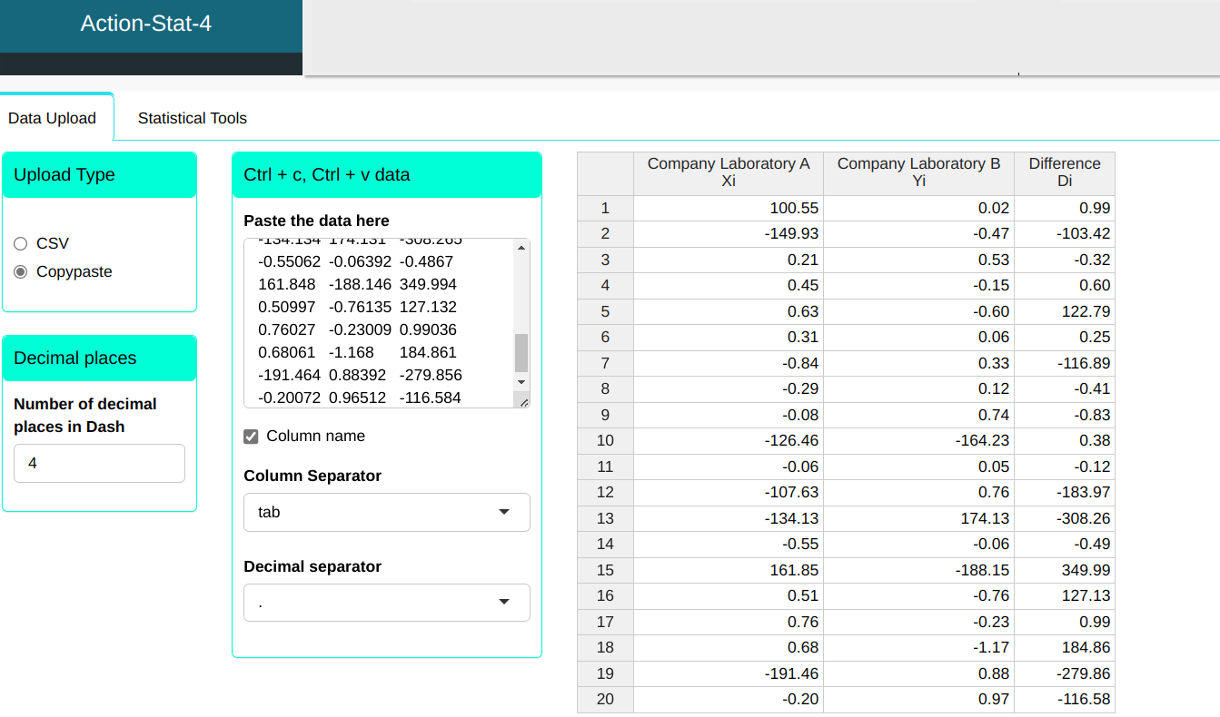
Consider $X_1, X_2, \ldots, X_20$ as a sample of measurements from the laboratory of Company A and $Y_1, Y_2, \ldots, Y_20$ as a sample of measurements from the laboratory of Company B. The tests of both laboratories are carried out in the same standard, so there is a correlation between them, that is, the samples are dependent. Evaluate the compatibility of the measurements between the laboratory of Company A and the laboratory of Company B.
| Laboratório da empresa A (Xi) | Laboratório da empresa B (Yi) | Diferença (Di) |
|---|---|---|
| 1.00552 | 0.01942 | 0.98610 |
| -1.49928 | -0.46512 | -1.03416 |
| 0.21367 | 0.53218 | -0.31851 |
| 0.44658 | -0.14844 | 0.59502 |
| 0.62766 | -0.60021 | 1.22787 |
| 0.31091 | 0.06495 | 0.24596 |
| -0.83878 | 0.33013 | -1.16891 |
| -0.29054 | 0.12116 | -0.41170 |
| -0.08487 | 0.74269 | -0.82756 |
| -1.26465 | -1.64232 | 0.37767 |
| -0.06353 | 0.05497 | -0.11850 |
| -1.07632 | 0.76342 | -1.83974 |
| -1.34134 | 1.74131 | -3.08265 |
| -0.55062 | -0.06392 | -0.48670 |
| 1.61848 | -1.88146 | 3.49994 |
| 0.50997 | -0.76135 | 1.27132 |
| 0.76027 | -0.23009 | 0.99036 |
| 0.68061 | -1.16800 | 1.84861 |
| -1.91464 | 0.88392 | -2.79856 |
| -0.20072 | 0.96512 | -1.16584 |
So, considering Di = Xi - Yi and establishing the hypotheses
- $H_0: \mu_D = 0$
- $H_0: \mu_D \neq 0$
where $\mu_D$ will be estimated by the sample mean of the differences, i.e. D. Using Action Basic Statistics tool, we find that the sample mean is D = -0.110499 and the sample standard deviation is S = 1.56907778.
We will upload the data to the system.
Configuring as shown in the figure below to perform the test.
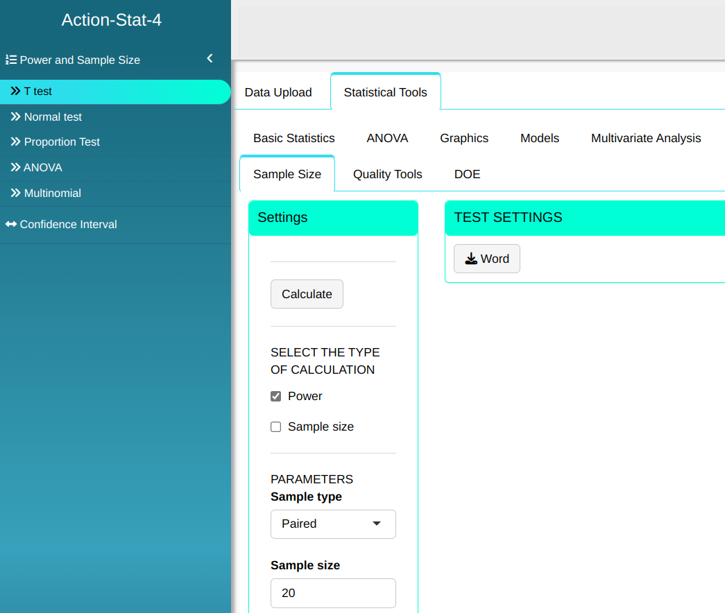
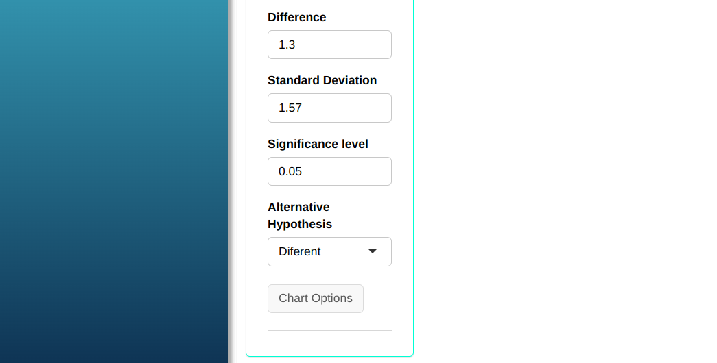
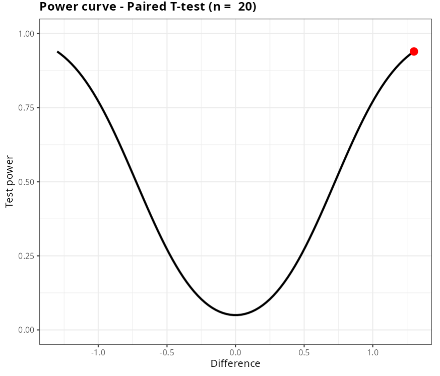
Then click Calculate we obtain the results. You can also generate the test and download them in Word format.
The results are:
T Test - Paired
| V1 | |
|---|---|
| Power | 0.9394575 |
| Sample size | 20 |
| Difference | 1.3 |
| Significance Level | 0.05 |
| Standard Deviation | 1.57 |
| Alternative Hyphotesis | Different |
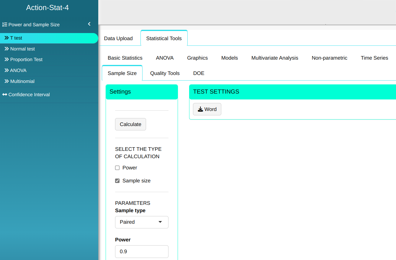
Example 8:
Using the previous example, now suppose we want to calculate the sample size needed for the Paired T-test to detect a difference of 0.5 with a power of at least 90%
Configuring as shown in the figure below to perform the test.

Then click Calculate we obtain the results. You can also generate the test and download them in Word format.
The results are:
Teste T - Pareado
| V1 | |
|---|---|
| Power | 0.9 |
| Sample Size | 106 |
| Difference | 0.5 |
| Standard Deviation | 1.57 |
| Significance Level | 0.05 |
| Alternative Hyphotesis | Different |
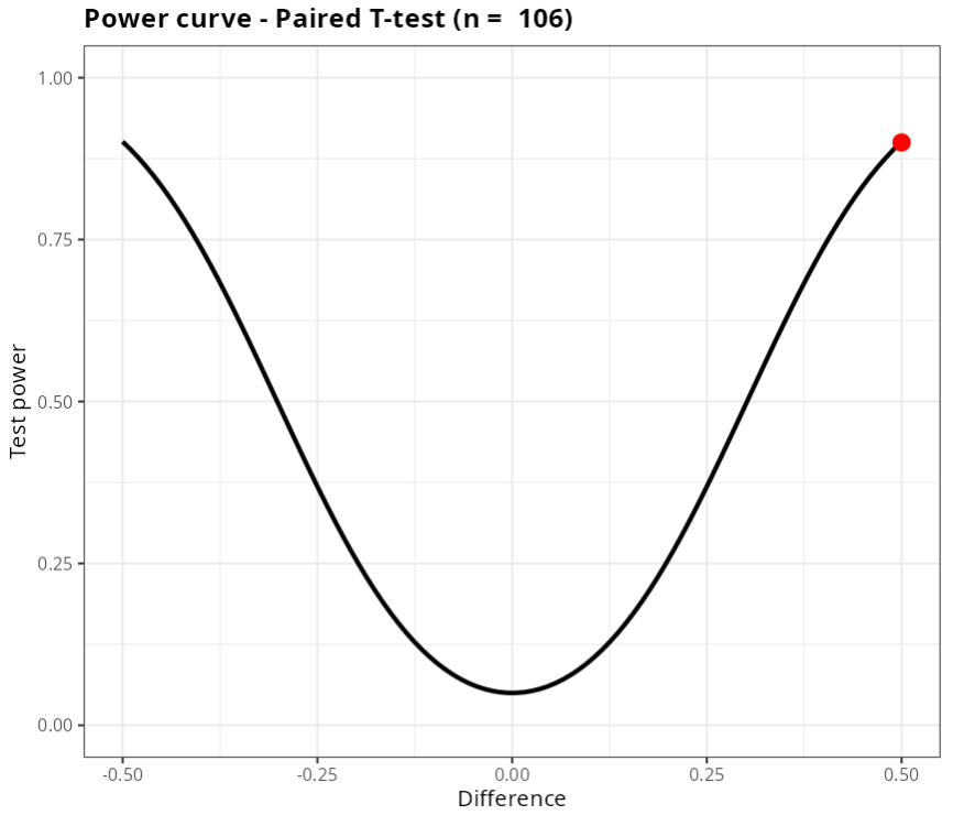
Therefore, for the test to detect a difference of 0.5 in the hypothesis test with a power of at least 0.9, a sample size of at minimum n = 106 is required.