1. Model Selection: Linear Model
The selection of a linear model can be evaluated by several factors that indicate the best model.
Example 1:
The gain of a transistor is the difference between the emitter and collector. The variable Gain (in hFE) can be controlled in the ion deposition process by means of the variables Emission time (in minutes) and Ion dose ( X $10^{14}$).
The aim is to evaluate the linear relationship between the transistor gain and the covariates emission time and ion dose.
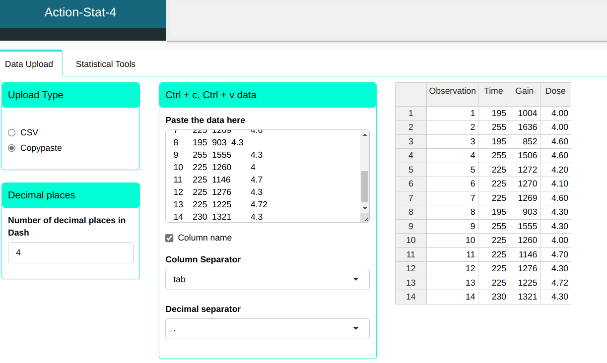
The data can be found in Table.
| Observation | Time | Dose | Gain |
|---|---|---|---|
| 1 | 195 | 4 | 1004 |
| 2 | 255 | 4 | 1636 |
| 3 | 195 | 4.6 | 852 |
| 4 | 255 | 4.6 | 1506 |
| 5 | 225 | 4.2 | 1272 |
| 6 | 225 | 4.1 | 1270 |
| 7 | 225 | 4.6 | 1269 |
| 8 | 195 | 4.3 | 903 |
| 9 | 255 | 4.3 | 1555 |
| 10 | 225 | 4 | 1260 |
| 11 | 225 | 4.7 | 1146 |
| 12 | 225 | 4.3 | 1276 |
| 13 | 225 | 4.72 | 1225 |
| 14 | 230 | 4.3 | 1321 |
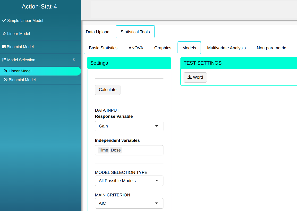
We will upload the data to the system.
Configuring as shown in the figure below to perform the analysis.
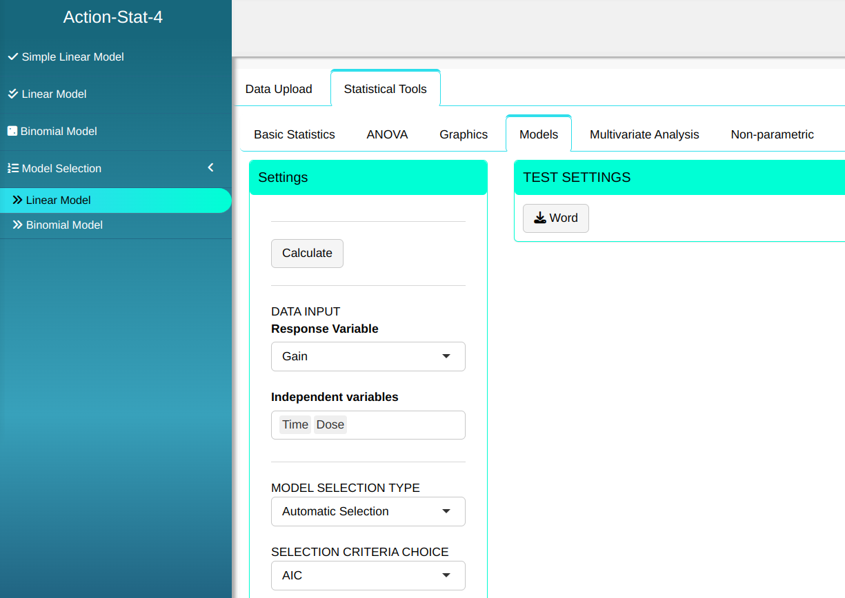

Then click Calculate to get the results. You can also generate the analyses and download them in Word format.
The results are:
Model Selection table
| Models (Pasos) | DF | Deviations(Deviance) | GL Residues | Deviance Residual | AIC | Choose |
|---|---|---|---|---|---|---|
| Gain~1 | 13 | 665387.21 | 152.7669 | |||
| Gain~Time | 1 | 630967.86 | 12 | 34419.35 | 113.3024 | |
| Gain~Time+Dose | 1 | 20998.23 | 11 | 13421.12 | 102.1174 | Selected model |
Model coefficients table
| Estimate | Standrad Deviation | T Stat. | P-value | |
|---|---|---|---|---|
| Intercept | -520.07668 | 192.1070916 | -2.707223 | 0.0203918463055154 |
| Time | 10.78116 | 0.4743196 | 22.729731 | 0 |
| Dose | -152.14887 | 36.6754390 | -4.148522 | 0.0016204993349917 |
Exploratory Analysis (residuals)
| Minimum | 1Q | Mean | Median | 3Q | Maximum |
|---|---|---|---|---|---|
| -44.584 | -26.348 | -3.266 | 0 | 26.004 | 63.201 |
Descriptive measure for Goodness-of-Fit
| Standard deviation of residuals | Degrees of Freedom | R^2 | adjusted R^2 |
|---|---|---|---|
| 34.92995 | 11 | 0.9798296 | 0.9761623 |
Example 2:
With the same data as Example 1, we will now apply the F-Test as a selection criterion.
The aim is to evaluate the linear relationship between the transistor gain and the covariates emission time and ion dose.
The data can be found in Table.
| Observation | Time | Dose | Gain |
|---|---|---|---|
| 1 | 195 | 4 | 1004 |
| 2 | 255 | 4 | 1636 |
| 3 | 195 | 4.6 | 852 |
| 4 | 255 | 4.6 | 1506 |
| 5 | 225 | 4.2 | 1272 |
| 6 | 225 | 4.1 | 1270 |
| 7 | 225 | 4.6 | 1269 |
| 8 | 195 | 4.3 | 903 |
| 9 | 255 | 4.3 | 1555 |
| 10 | 225 | 4 | 1260 |
| 11 | 225 | 4.7 | 1146 |
| 12 | 225 | 4.3 | 1276 |
| 13 | 225 | 4.72 | 1225 |
| 14 | 230 | 4.3 | 1321 |
We will upload the data to the system.
Configuring as shown in the figure below to perform the analysis.
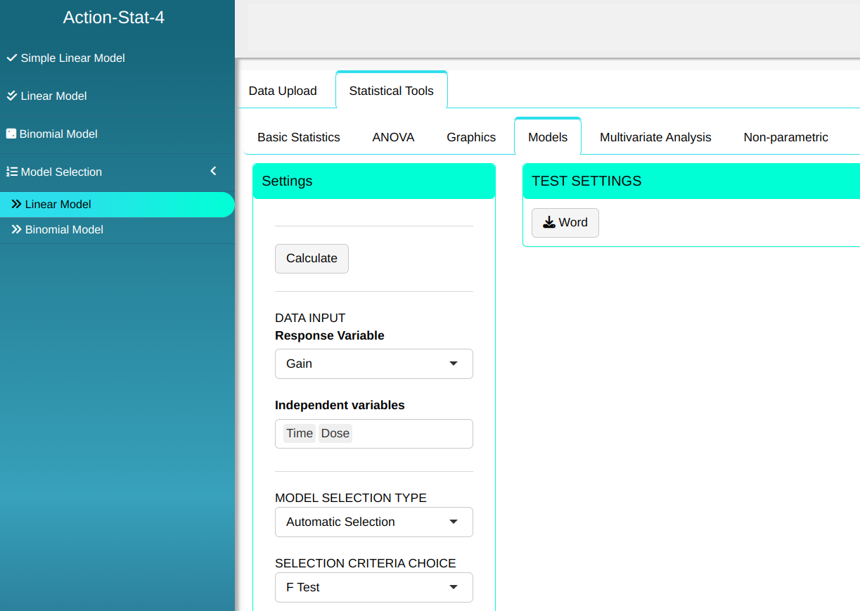

Then click Calculate to get the results. You can also generate the analyses and download them in Word format.
The results are:
Model Selection table
| Modelo(Steps) | Variable In | Variable Out | Statistic F | P-Value |
|---|---|---|---|---|
| Model 1 | Tempo | 219.98133 | 4.421162e-09 | |
| Model 2 | Dose | 17.21024 | 1.620499e-03 | |
| Selected Model | Time + Dose |
ANOVA Table
| D.F. | Sum of Squares | Mean Squares | F Stat. | P-value | |
|---|---|---|---|---|---|
| Time | 1 | 630967.8649 | 630967.8649 | 517.1438 | 0 |
| Dose | 1 | 20998.234 | 20998.234 | 17.2102 | 0.0016 |
| Residuals | 11 | 13421.1153 | 1220.1014 |
Example 3:
With the same data as Example 1, instead of automatically selecting the models, the three best ones will be chosen from all possible options.
The aim is to evaluate the linear relationship between the transistor gain and the covariates emission time and ion dose.
The data can be found in Table.
| Observation | Time | Dose | Gain |
|---|---|---|---|
| 1 | 195 | 4 | 1004 |
| 2 | 255 | 4 | 1636 |
| 3 | 195 | 4.6 | 852 |
| 4 | 255 | 4.6 | 1506 |
| 5 | 225 | 4.2 | 1272 |
| 6 | 225 | 4.1 | 1270 |
| 7 | 225 | 4.6 | 1269 |
| 8 | 195 | 4.3 | 903 |
| 9 | 255 | 4.3 | 1555 |
| 10 | 225 | 4 | 1260 |
| 11 | 225 | 4.7 | 1146 |
| 12 | 225 | 4.3 | 1276 |
| 13 | 225 | 4.72 | 1225 |
| 14 | 230 | 4.3 | 1321 |
We will upload the data to the system.
Configuring as shown in the figure below to perform the analysis.

Then click Calculate to get the results. You can also generate the analyses and download them in Word format.
The results are:
Model Selection table
| V1 | AIC | CP | R^2 | adjusted R^2 | BIC | PRESS | QME | |
|---|---|---|---|---|---|---|---|---|
| X2 | Time + Dose | 143.848 | 3 | 0.98 | 0.976 | 146.404 | 22225.01 | 1220.1014 |
| X1 | Time | 155.033 | 18.21 | 0.948 | 0.944 | 156.95 | 51545.126 | 2868.2791 |
| X1.1 | Dose | 196.035 | 517.641 | 0.032 | -0.048 | 197.952 | 875529.652 | 53647.9287 |